The Atmospheric Response to Realistic Reduced Summer Arctic Sea Ice Anomalies - Arctic Sea Ice Decline: Observations, Projections, Mechanisms, and Implications - page 90

put using a linear baroclinic model (LBM) to show that the
initial local response is baroclinic and forced by the diabatic
heating anomalies associated with surface heat fluxes result-
ing from reduced sea ice area. The equilibrium response is
large scale in extent, barotropic, and primarily maintained
by the transient eddy vorticity fluxes. Peng and Whittaker
[1999] elucidated this eddy-driven mechanism to describe
the atmospheric response to midlatitude SSTs in an idealized
GCM, which can be applied to surface changes resulting
from decreased sea ice. These studies show that the atmo-
sphere responds to surface boundary conditions in ways that
can influence the storm track.
Alexander et al. [2004] forced CCM3 with realistic sea
ice conditions, characterized by negative (positive) ice ex-
tent anomalies east (west) of Greenland, from 1982 to 1983
that had a similar pattern but with a smaller ice area than the
anomalies from Magnusdottir et al. [2004] and Deser et al.
[2004]. The pattern of response is similar in the three stud-
ies, with positive (negative) height anomalies in the Arctic
(midlatitudes). A comparison of ice area to the strength of
500-hPa response reveals a linearly increasing relationship
[see Alexander et al. , 2004, Figure 9].
Alexander et al. [2004] also examined the response to
ice anomalies in the North Pacific and found that the atmo-
spheric response suggested a positive feedback of the ice on
the atmosphere. The different atmospheric responses to ice
in the North Atlantic and North Pacific may arise from the
position of the storm track relative to the ice edge. In the

North Atlantic the ice edge is in the vicinity of the storm
track, whereas in the North Pacific the ice edge is well north
of the storm track. A thorough discussion of additional stud-
ies of the response to winter sea ice is presented by Alexan-
der et al. [2004].
Numerous GCm simulations have investigated the impact
of winter sea ice on the atmosphere but few have examined
the atmospheric response to sea surface temperature or sea
ice during the summer months. Several studies find the re-
sponse during summer to be much weaker than winter and
focus their analysis on winter [ Parkinson et al. , 2001; Sin-
garayer et al. , 2006]. Raymo et al. [1990] reduced the ice
to paleoclimatic conditions throughout the year that reached
an ice-free Arctic during the month of September. During
June, July, and August (JJA) they found a 3°K warming over
Greenland and an overall warming over the polar region.
They found no significant differences in sea level pressure,
evaporation/precipitation ratios, or cloudiness in the North
Atlantic.
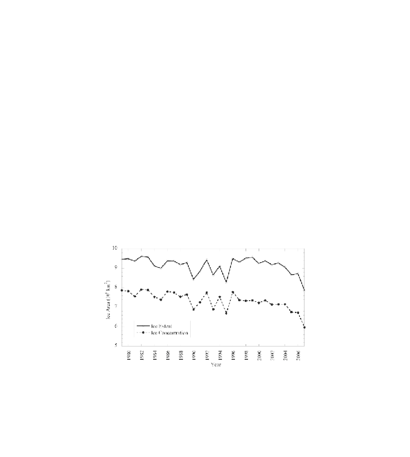
This study employs CCM3 to investigate the atmospheric
response to reduced realistic summer sea ice in the Arctic
from the summer of 1995, which had the lowest June-Sep-
tember ice area (based on both extent and concentration)
with the exception of the summer of 2007 (Figure 1). Note
that the sea ice minimum in September has been close to or
well below the 1995 levels since 2002 [ Stroeve et al. , 2008].
In addition to using realistic sea ice extents and concentra-
tions in the Arctic, the other unique features of our study

Figure 1. Observed Arctic-wide ice cover (multiplied by 10 6 km 2 ) based on ice extent (solid line) and concentration
(dashed line) during summer (June-September) over the period 1979-2007 in the HadISST1 1° ´ 1° data set. Ice is
defined to extend over a grid square when the ice concentration is 15% or greater. The summer of 1995 had the overall
minimum June-September ice extent with the exception of 2007, which was significantly lower.