Reconstructing Sea Ice Conditions in the Arctic and Sub-Arctic Prior to Human Observations - Arctic Sea Ice Decline: Observations, Projections, Mechanisms, and Implications - page 31

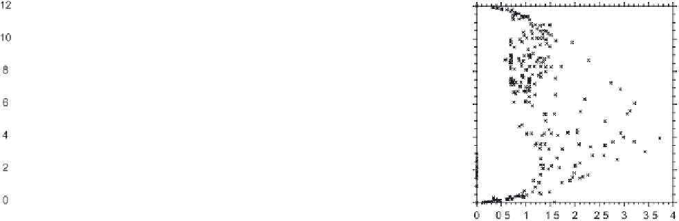
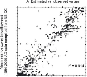
Figure 3. Illustration of the accuracy of the modern analogue technique (MAT) applied to dinocyst assemblages for
estimating past sea ice cover extent: (a) estimated versus observed sea ice for the 1954-2000 A.D. time interval at refer-
ence sites; (b) distribution of the residuals, which are the differences between observed and estimated values, versus the
mean sea ice cover for the 1954-2000 A.D. time interval; and (c) standard deviation (1σ) of the 1954-2000 A.D. sea ice
cover extent at the reference sites versus the mean sea ice cover for the 1954-2000 A.D. time interval. All values are
expressed in terms of months per years of sea ice cover with concentration greater than 50% at given sites defined on a
1° by 1° grid scale. In Figure 3a, the RMSe is the root mean square error, which corresponds to the standard deviation
of the residual.

may reach 3.7 months/year but averages ±1.0 month/year
(Figure 3c).

ancy in the sea ice cover from the time interval included in
the surface sediments (hundreds of years) and that of the last
decades. On the average, dinocyst estimates that represent
the last hundreds of years suggest less sea ice than during the
last decades along the eastern Greenland margin (Figure 4).
In the northern Barents Sea, dinocyst assemblages also yield
underestimated sea ice cover values, but the assemblages
south of the maximum sea ice limit provide overestimations.
Such anomalies might reflect a more southward spread of
sea ice in winter, and a reduced summer sea ice cover in the
northern area of the eastern Barents Sea, during the previous
centuries. If the above interpretation of the residuals is cor-
rect, the mean state of sea ice cover at secular scales could
have been more zonal in the Nordic seas and with a less pro-
nounced west to east gradient than at present. However, such
an interpretation has to be considered with caution because
of intrinsic limitations of the transfer function and because
the MAT approach is an interpolation technique that might
result in some smoothing. In any case, the spatial pattern of
the residuals deserves some attention and points to the fact
that secular time series with decadal resolution are needed to

3.3. Variability and Secular Changes in Sea Ice Cover

The spatial distribution of the residuals (Figure 4), which
are the differences between observed and estimated values
of sea ice cover, may provide additional information on the
reliability of reconstructions. Residuals are relatively high
in ice marginal zones such as the eastern Greenland margins
and the Barents Sea, which are also areas of high interan-
nual variability as seen in observation data compiled for the
1954-2000 A.D. period (Figure 5). Therefore, we have to
admit some uncertainty in reconstructions due to both the
reliability of the transfer function and the inherent high vari-
ability of sea ice cover at the sea ice margin.
A closer examination of the geographical distribution
of residuals shows interesting features. Along the eastern
Greenland margins, within the limit of the mean sea ice edge,
dinocyst data consistently yield underestimated sea ice cover
values. This illustrates a bias that may result from a discrep-

Figure 2. (Opposite) Results of canonical correspondence analyses performed on the dinocyst assemblages (64 taxa) and surface ocean
parameters (sea ice, temperature, salinity, and productivity) using the Canoco software [cf. ter Braak and Smilauer , 1998]. Sea ice stands
as (top) a determinant parameter on the assemblage distribution at the scale of the Northern Hemisphere and as (bottom) the most deter-
minant parameter at the scale of the Arctic data set (north of 66°N, see dark gray squares in Figure 1), which includes 401 sites and 37
dinocyst taxa. Details on the data treatments are reported elsewhere [ Radi and de Vernal , 2008].