What Is the Trajectory of Arctic Sea Ice? - Arctic Sea Ice Decline: Observations, Projections, Mechanisms, and Implications - page 176

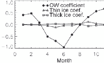
Figure 6. Coefficients of the sum of equations (2): open water (OW)
coefficient a ( t ) + d ( t ) (circles), thin ice coefficient b ( t ) + e ( t ) (triangles),
and thick ice coefficient c ( t ) + f ( t ) (squares).

(0,0), with decreasing amounts of thin ice nearly every year.
The annual cycle for 2044 is shifted downward relative to
2005, i.e., less thick ice, but there is also a noticeable change
in the shape of the annual cycle: (1) In 2044 there is a loss of
thin ice from june to july, whereas in 2005 and earlier years
there is a gain of thin ice. (2) In 2044 the loss of thin ice from
july to August is far greater than in the earlier years. This
might be understood as follows:
1. When there is a relatively large amount of thick ice in
june, and it begins to melt, it creates thin ice faster than the
thin ice itself can melt. But when there is relatively little
thick ice in june, its conversion to thin ice cannot keep up
with the melting of the thin ice itself.

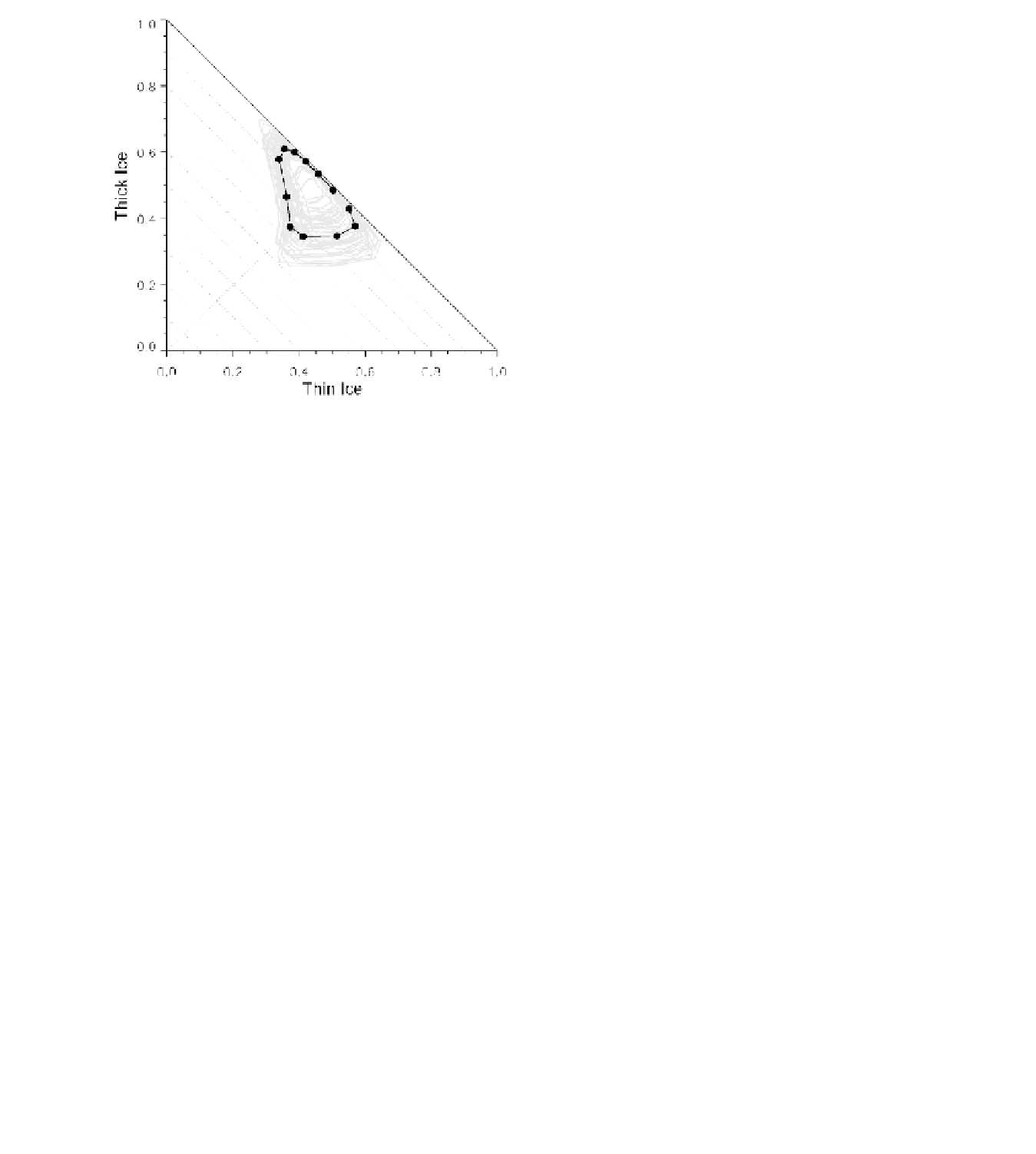
Figure 5. Monthly values of the equilibrium trajectory (circles)
obtained by integrating equations (2). The 48-year PIOMAS trajec-
tory is shown in gray.

The periodicity of the coefficients allows for an annual cycle
of thin ice and thick ice. There is no interannual variability
in this empirical model. The point of this two-dimensional
exercise is that a simple linear model can reproduce the an-
nual cycle of thin ice and thick ice fairly well, and it has one
stable state: the trajectory always converges to that of figure
5 no matter what the initial condition. It will never evolve to
an ice-free Arctic.
If we add together equations (2), we obtain a single equa-
tion for the total ice concentration, z = x + y , of the form d z /d t =
( a + d )(1 - z ) + ( b + e ) x + ( c + f ) y . On the basis of the one-
dimensional case above, we would expect a + d to be approxi-
mately a cosine function with amplitude close to 1, and b + e
and c + f should be zero or small. This is indeed the case, as
shown in Figure 6. This confirms that the two-dimensional
model is consistent with the one-dimensional model.
A trend in external forcing (such as increasing atmo-
spheric CO 2 ) is capable of driving the trajectory of Arctic
sea ice toward a state with ice-free summers, according to
the recent predictions of several models [ Zhang and Walsh ,
2006]. figure 7 shows the trajectory of the CCSM3 model
for 150 years (1950-2099). The annual cycles through 2005
are similar to those from PIOMAS (figure 3). from 1950
through about 2005, the amount of thick ice in September
decreases but the amount of thin ice in September is fairly
constant. After 2005 the September trajectory swings toward

Figure 7. Trajectory of the CCSM3 model for 150 years, 1950-
2099 (gray). Monthly values are shown for the years 1966, 2005,
2044, and 2083.