Multiple Equilibria and Abrupt Transitions in Arctic Summer Sea Ice Extent - Arctic Sea Ice Decline: Observations, Projections, Mechanisms, and Implications - page 149

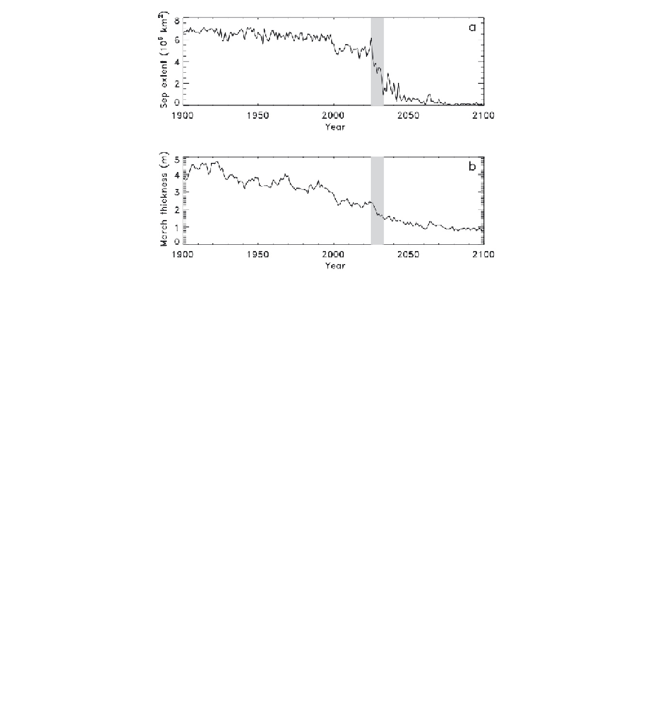
Figure 1. Time series of 20th and 21st century (a) September ice extent and (b) mean March ice thickness, as represented
by a single realization of CCSM3 under the Special Report on Emissions Scenarios A1b forcing scenario. The gray bands
represent an interval of abrupt decrease in ice extent as defined in the text.

only, is unstable. This “all or nothing” situation resembles
the SICI phenomenon described by North [1984].
Flato and Brown [1996] applied a local thermodynamic
ice model derived from that of Maykut and Untersteiner
[1971] to study climate sensitivity of landfast Arctic sea ice.
The model contains detailed parameterizations of ice prop-
erties and includes effects of snow. When subject to an an-
nual cycle of forcing derived from observations, the model
exhibits two distinct equilibria, one consisting of perennial
ice having a modest seasonal cycle in thickness and the
other seasonally ice free. These solutions are separated by a
third, unstable equilibrium having intermediate annual mean
thickness [ Flato and Brown , 1996, Figure 8c].
An intermediate level of complexity is represented by the
investigation of Björk and Söderkvist [2002]. Their model
is closer to a column version of a comprehensive climate
model, with ice cover described by a thickness distribution,
a prognostic one-dimensional ocean having a dynamic ocean
mixed layer and parameterized lateral ocean transports, and
an atmospheric model built on that of Thorndike [1992].
Forcing is provided by monthly means of observed clima-
tological quantities. like the simpler model of Thorndike
[1992], it exhibits dual equilibria having perennial ice in one
instance and no ice cover in the other.

Finally, in a more idealized context, Taylor and Feltham
[2005] treated sea ice as a floating slab subject to surface
heating by solar radiation and cooling by other processes.
A simple radiative transfer model was used to represent ra-
diative penetration and associated internal heating. The ice
thickness equilibria, determined analytically, consist of a
stable solution branch that decreases with increasing inci-
dent shortwave flux, until a critical flux is reached. At that
point an infinitesimal further increase in shortwave flux
results in collapse from finite to zero thickness. The disap-
pearance of the stable equilibrium occurs through its merger
with an unstable solution branch [ Taylor and Feltham , 2005,
Figure 6].

2.3. Climate System Box Models

As a means for studying climate system evolution over
very long timescales, Gildor and Tziperman [2001] devised
a coupled box model comprising a planetary domain divided
into four latitude bands, with both sea ice and ice sheets on
land included. Their main finding was that growth of sea
ice cover in a cooling climate reduces the atmospheric sup-
ply of moisture to ice sheets, resulting in a negative feed-
back that leads, in turn, to glacial cycle-like oscillations on a