Biomedical Engineering Reference
In-Depth Information
0.08
400
0.06
0.04
200
0.02
0
0.00
0
100
Displacement / nm
50
150
0
100 200
Debonding force (pN)
300
400
500
600
A
B
0 µm
23 µm
0 µm
23 µm
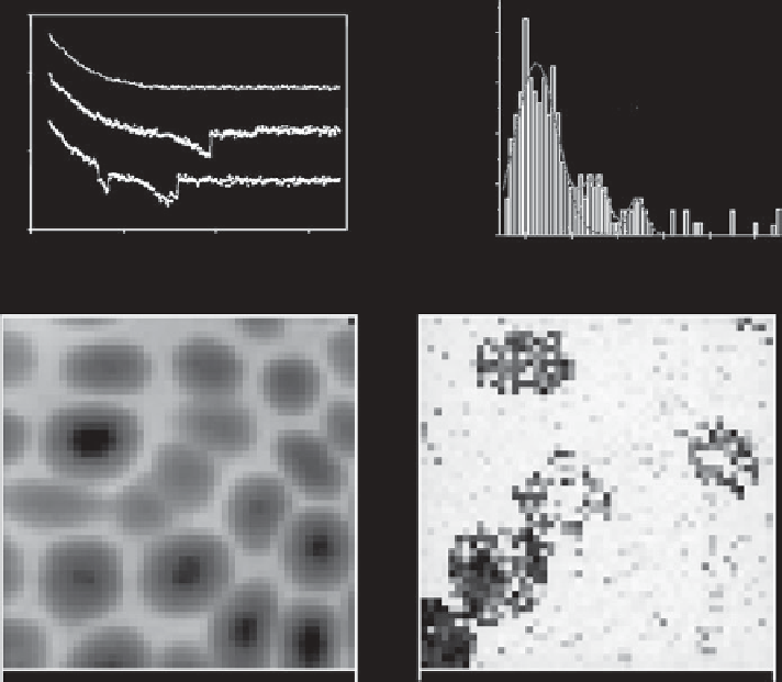
Fig. 7.26. Examples of biological force spectroscopy. The two examples show different methods of
studying interactions with human blood cells - at the top, one-dimensional force spectroscopy, and
below, three-dimensional force mapping. Top: force spectroscopy on human platelets. The top
force-distance curve was made with an unmodified tip, and the bottom two with a tip modified
with peptide sequences from fibrinogen, showing the results of single (middle curve) and multiple
(lower curve) adhesion events. On the right is a 'force spectrum', showing the presence of peaks at
multiples of
ca
. 93 pN. Below: force mapping on red blood cells with a lectin-modified probe. Image
A is the total adhesion force and image B is the topography of a mixed layer of group A and O cells.
The topography shows no difference between the cells, while the adhesion image clearly distin-
guishes 'A' from 'O'. Adapted from [688] and [710].
AFM instrument approaches the probe to contact the surface, and then pulls the probe
away, before moving a small amount while out of contact, approaching again, etc. This is
done in a grid pattern defined by the user. This method of measuring interactions has great
advantages in that the individual force curves are as well-defined and controllable as via
normal (1-D) force spectroscopy, and are carried out normal to the sample surface.
However, it is also a rather slow technique, and normally the maps are produced with
reduced resolution (e.g. 64
64 points [142]), in order to make the experiments reason-
ably short. In addition, the data processing can be complicated and time-consuming.