Biomedical Engineering Reference
In-Depth Information
0 nm
17 nm
-5 nm
0 nm
5 nm
0 nm
-5 nm
0 nm
5 nm
17 nm
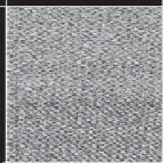
Fig. 5.13. Example of autocorrelation analysis. Left: unfiltered noisy image of an atomic lattice.
Right: 2-D autocorrelation function derived from the image. Note the change in scale; the origin
moves to the centre of the image, because the result is not an image, but rather it's a plot of self-
correlation in the source image. Typically, the centre will be clearest, showing short-range correl-
ation; long-range correlation is required for the outer regions to have the same amplitude.
also a very powerful filtering method. For example, one might be able to use this method
to remove noise at any particular frequency from an image. Other examples include
removal of streaking in images of soft samples [374]. However, one must be very careful
in interpretation of Fourier-filtered images; it is easy using to such a method to artificially
create an image with any desired pattern, even one that never existed in the original
un-filtered data; see the lower part of Figure 5.12.
Autocorrelation analysis is another method for the analysis of repeating patterns in data.
Outside of AFM, one-dimensional autocorrelation is most popular, but for AFM images,
two-dimensional autocorrelation is more useful. Two-dimensional autocorrelation of an
image results in an image containing the periodic patterns present in the original image,
with spontaneous (non-repeating) features removed. Unlike the Fourier transform image,
the autocorrelation function is shown in real space, so the spacing of the repeating features
can then be measured directly from the image. Like FFT analysis, a common application
for autocorrelation analysis in AFM is measurement of atomic lattice spacing. An example
of two-dimensional autocorrelation analysis is shown in Figure 5.13.