Environmental Engineering Reference
In-Depth Information
100
2.55
(a)
Surface runoff
Total stream flow
1.98
10
1.42
B
Baseflow
A
0.85
1
2.55
(b)
Base flow
Surface runoff
1.98
C
0.1
012345678910
11
12
1.42
Days
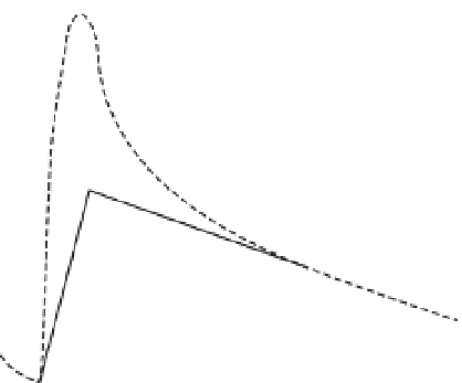
Figure 4.8
Schematic showing steps in manual
hydrograph separation; A marks the point in time after
which the recession curve becomes approximately linear,
B is the time of the first inflection point on the hydrograph
after the peak, and C is the point of initial rise in the
hydrograph. Base flow for the hydrograph rise is calculated
as the area under the line segments AB and BC.
Baseflow
0.85
2.55
(c)
Surface runoff
1.98
1.42
Recent advances in computer programs for
automatically performing hydrograph sep-
aration have greatly facilitated the process,
removing much of the subjectivity, reducing
the amount of time required for analysis, and
allowing analyses of complex hydrographs
(Pettyjohn and Henning,
1979
; Institute of
Hydrolog y,
1980
; Wahl and Wahl,
1988
; Nathan
and McMahon,
1990
; Rutledge,
1998
; Arnold
et al
.,
1995
; Arnold and Allen,
1999
; Sloto and
Crouse,
1996
; Lim
et al
.,
2005
). Approaches
vary among these models, but they all employ
some empirical formula or low-frequency fil-
ter for separating base flow from the stream-
flow hydrograph. Two of the methods are
described here.
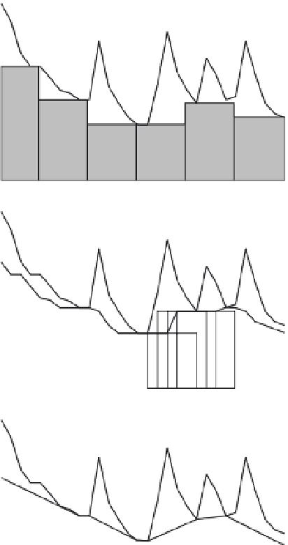
The HYSEP computer program (Sloto and
Crouse,
1996
) offers three separate algorithms
for hydrograph separation; all three were ori-
ginally described by Pettyjohn and Henning
(
1979
): local minimum, fixed interval, and slid-
ing interval. Conceptually, these algorithms
provide alternative approaches to connecting
Baseflow
0.85
1
5
10
15
20
25
30
April 1992
Figure 4.9
Hydrograph separation for French Creek
near Phoenixville, Pennsylvania, April 1992, as determined
from the HYSEP computer program using (a) fixed-interval,
(b) sliding-interval, and (c) local-minimum methods (Sloto
and Crouse,
1996
).
lines between low points of the streamflow
hydrograph (
Figure 4.9
). The first step is to esti-
mate the length of time following peak dis-
charge over which surface flow continues to
contribute to streamflow. A common assump-
tion is that the length of this time interval,
N
, is
constant for all flows and that it can be approxi-
mated (Linsley
et al
.,
1982
) as:
N
=
0.83
A
0.2
(4.6)