Environmental Engineering Reference
In-Depth Information
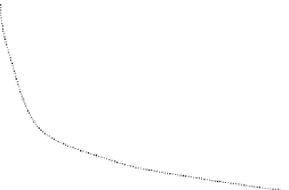
Max. gradient power
P
Power
300
T
90 kW
250
80 kW
70 kW
200
60 kW
150
50 kW
40 kW
100
30 kW
50
20 kW
g/kWh
10 kW
0
0
500
1,000
1,500
2,000
2,500
3,000
3,500
4,000
Engine speed (rpm)
Figure 1.36 ICE fuel consumption mapping into torque-speed plane
vehicle fuel economy calculated with the aid of a fuel island map as shown in
Figure 1.36 can be taken as
5,250
V
avg
g
BSFC
P
trac
avg
FE
mpg
¼
ð
1
:
44
Þ
where vehicle speed,
V
avg
, is in mph, BSFC in g/kWh and traction power in kW.
For example, in (1.44) assume the vehicle is travelling in the city at 35 mph for a
road load of 12 kW and consumes 480 g/kWh of fuel for the particular transmission
gear and final drive ratios. This yields an FE of 32 mpg. If the driveline gear ratios
are such that the same conditions are met at lower engine speed along a constant
power hyperbola, the BSFC decreases to 350 g/kWh, improving the fuel economy
to 43 mpg.
When the engine torque moves upwards along a constant power contour, the
engine is said to be lugging. That is, the same power output is delivered but at lower
engine speeds and higher torques. Lugging is typically a more fuel efficient engine
state. More will be said of lugging and driveline gear ratio selection in Chapter 3.
1.7.4 Emissions regulations
As this second edition of
Propulsion Systems for Hybrid Vehicles
is being written,
legislation is going into place across the globe to substantially increase vehicle fuel
economy standards. Earlier sections have highlighted the need for CO
2
reduction
and some of the technologies that facilitate reaching 30-50% CO
2
reductions (see
Figure 1.12). Here we take a look at recent developments in emissions legislation
and vehicle impacts.