Environmental Engineering Reference
In-Depth Information
determines charge flow, which in turn defines the exchange current,
I
0
, as shown
in (10.6):
RT
nF
ln
ð
I
=
I
0
Þ
V
Þ
E
a
¼
ð
10
:
6
Þ
Equation (10.6) can be rewritten as a linear equation from which a Tafel plot
can be constructed:
E
¼
a
b
log
ð
I
Þ
V
Þ
ð
10
:
7
Þ
2.303
RT
/
a
nF
2
where
a
is a constant,
b
~0.5 the charge transfer coef-
ficient. By extrapolating (10.7) to zero in the Tafel plot, the value of the equili-
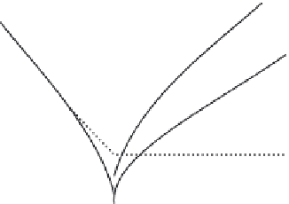
brium exchange current at the given system temperature is obtained. An example of
a Tafel plot is given in Figure 10.3 for representative charge transfer coefficients.
Activation polarization has relatively fast time dynamics for build-up and decay.
¼
and
a
¼
Log (
I
)
a
2
1-
a
1
a
1
1-
a
2
I
0
Potential
E
eq.
Figure 10.3 Charge-potential behaviour of a cell electrode
Concentration polarization
is strongly dependent on the supply of reactants in
the cell and how the by-products are removed or displaced. This effect is defined
in (10.8), where
C
is the concentration in solution and
C
e
is the concentration of the
electrolyte at the electrode surface, both in units of mol/L or mol/cm
3
:
ð
V
Þ
RT
nF
ln
C
e
C
E
c
¼
ð
10
:
8
Þ
2
The reader will recognize that a logarithmic base change was used:
b
ln(
M
)=
b
log(
M
)
ln(10) =
2.3026
b
log(
M
).