Essential Statistical Concepts, Definitions, and Terminology - Sampling Spatial Units for Agricultural Surveys - page 21

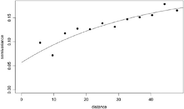
Fig. 1.1 Empirical semivariogram ( points ) and fitted model ( dashed line )

Now, assume that a spatial random field for geostatistical data can be expressed

as

y z ðÞ ¼ ʼ z ðÞþʵ z ðÞ , ε ðÞ/ 0 ð ; ʣ Þ; ð 1 : 40 Þ

where (z i ) is white noise with

zero mean. The mean function represents the systematic component of the spatial
process, and considers the large-scale variations. The error term takes into account
local irregularities, and considers small-scale variations.
We may be interested in estimating the mean value (i.e., a global estimate for the
whole region under investigation). However, predicting y (z) at unobserved loca-
tions is often a more important issue in geostatistical applications.
Consider an un-sampled location z 0 . The main aim of geostatistics is to predict y
(z 0 ). It would seem reasonable to estimate y (z 0 ) using a weighted average of the
values at observed locations y (z i ), i ¼1,2,.., n , with weights given by some decreas-
ing function of the distance between the unobserved and observed sites. So, the
predictor of y (z 0 ) can be defined as

ʼ (z i ) is the mean of the spatial process, and the error ʵ

y z ðÞ ¼ X i ʻ i y z ðÞ: ^ ð 1 : 41 Þ

A simple and popular spatial prediction method is kriging. This method uses a
model of spatial continuity, or dependence.
The main purpose of kriging is to optimally determine the weights

ʻ i . A predictor
is defined by first constructing a function that measures the loss sustained by using y

(z 0 ) as a predictor of y (z 0 ). The squared loss function is most often used in practical
applications. Generally, the theory aims at finding estimators that minimize the
average loss. In this case, the loss can be expressed in terms of the mean squared
prediction error (MSPE) as

^