Graphics Reference
In-Depth Information
No
No
No
LDS
No
No
o
o
N
No
o
o
N
N
N
N
N
N
N
No
N
N
N
N
N
N
N
N
N
N
N
No
Stage 0
SIMD lane 0
Stage 0
SIMD lane 0
Stage 1
SIMD lane 1
Stage 1
SIMD lane 1
Stage 2
SIMD lane 2
Stage 2
SIMD lane 2
Stage 3
SIMD lane 3
Stage 3
SIMD lane 3
Yes
Yes
Yes
Yes
Yes
Y
e
Yes
Y
e
e
Yes
Y
Y
e
e
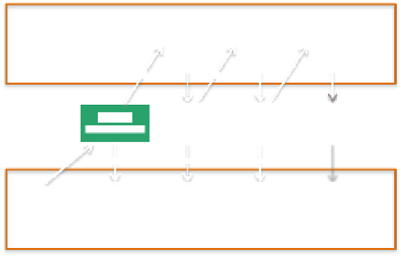
Global Memory
Figure 4.4.
Pipelined local batching.
Pipelined local batching always creates the same batches as serial batching,
whereas other parallel batching using atomics usually creates different batches
and the number of batches is greater than the number created by the serial algo-
rithm. Keeping the number of batches small is important to keep the computation
time of the expensive constraint solver low, as discussed in Section 4.2.
OpenCL kernel code for pipelined batching can be found in Listing 4.1.
4.4.3 Constraint Solver
The constraints are solved by four subsequent kernel executions: one kernel ex-
ecution for each set of constraint groups. Each dispatch assigns a SIMD for a
constraint group within a set, and batched constraints are solved in parallel by
checking batch indices. While the global constraint solver dispatches a kernel for
each batch, the two-level constraint solver always executes four kernels in which
a SIMD of the GPU repeats in-SIMD dispatches by itself until all the constraints
belonging to the group are solved.
4.5 Comparison of Batching Methods
A batching method can be evaluated by two aspects: batching computation time
and the performance of the constraint solver. Batching computation time is
shorter when local batching is used because it can be executed in parallel and
it needs to create batches only with the hardware SIMD width, while global
batching must create batches with the processor width (the SIMD width times
the number of SIMDs on the hardware).