Graphics Reference
In-Depth Information
Level 4
Level 3
Level 2
Level 1
Level 0
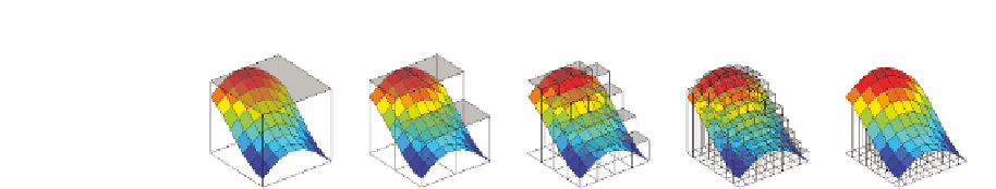
Figure 4.7.
The Hi-Z (Hierarchical-Z) buffer, which has been unprojected from screen
space into world space for visualization purposes. [Image courtesy of [Tevs et al. 08].]
Unlike the previously developed methods, which take constant small steps
through the image, the marching method we investigate runs much faster by
taking large steps and converges really quickly by navigating in the hierarchy
levels.
Figure 4.7 shows a simple Hierarchical-Z representation unprojected from
screen space back into world space for visualization purposes. It's essentially
a height field where dark values are close to the camera and bright values are
farther away from the camera.
Whether you construct this pass on a post-projected depth buffer or a view-
space Z-buffer will affect how the rest of the passes are handled, and they will
need to be changed accordingly.
4.4.2 Pre-integration Pass
The pre-integration pass calculates the scene visibility input for our cone-tracing
pass in a hierarchical fashion. This pass borrows some ideas from [Crassin 11],
[Crassin 12], and [Lilley et al. 12] that are applied to voxel structures and not
2.5D depth. The input for this pass is our Hi-Z buffer. At the root level all of our
depth pixels are at a 100% visibility; however, as we go up in this hierarchy, the
total visibility for the coarse representation of the cell has less or equal visibility
to the four finer pixels:
Visibility
n
≤
Visibility
n−
1
.
(See also Figure 4.8.) Think about the coarse depth cell as a volume containing
the finer geometry. Our goal is to calculate how much visibility we have at the
coarse level.
The cone-tracing pass will then sample this pre-integrated visibility buffer
at various levels until our ray marching accumulates a visibility of 100%, which
means that all the rays within this cone have hit something. This approximates
the cone footprint. We are basically integrating all the glossy reflection rays. We
start with a visibility of 1.0 for our ray; while we do the cone tracing, we will keep
subtracting the amount we have accumulated until we reach 0.0. (See Figure 4.9.)