Graphics Reference
In-Depth Information
Finally, loop variable
s
now runs from 1 to
N
Steps
inclusively and Prev
ρ
RM
,
Prev
dL
Rlgh
,andPrev
dL
Mie
variables are initialized by appropriate values for
camera position
C
before entering the loop. Trapezoidal integration requires
fewer steps to achieve the same precision. We found out that
N
Steps
=7are
enough to provide good refinement results. After coarse in-scattering is calculated
for each sample, we search for discontinuities and place additional ray marching
samples directly before and after each one. This algorithm is implemented with
the compute shader as described in Section 2.8.
2.7 1D Min/Max Binary Tree Optimization
2.7.1 General Idea
At this point we have selected a number of ray marching samples on each epipolar
line and need to compute the in-scattering integral for each one taking shadowing
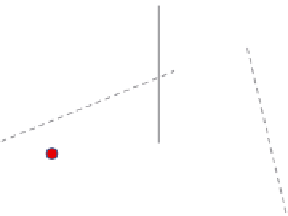
into account. For each sample, we cast a ray, then transform its start and end
positions into the light projection space and perform ray marching in shadow
map space (Figure 2.4).
Stepping through each shadow map texel would be too expensive, especially
for a high-resolution shadow map. Using a fixed number of samples can cause
undersampling and result in banding artifacts. We took advantage of epipolar
geometry to improve performance without sacrificing visual quality. Consider
camera rays casted through ray marching samples on some epipolar line (Fig-
ure 2.5). The rays clearly lie in the same plane, which we will call epipolar slice.
The most important property of the slice is that the light direction also belongs
to it.
The intersection of an epipolar slice with the light projection plane is a line.
All camera rays in the slice project to this line and differ only in the end point.
Shadow map
Figure 2.4.
Projecting the view ray onto the shadow map.