High Performance Outdoor Light Scattering Using Epipolar Sampling - GPU Pro: Advanced Rendering Techniques - page 109

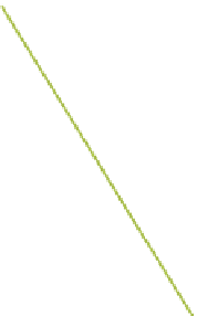
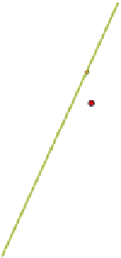
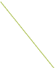
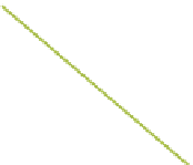
Ray marching sample Interpolation sample Epipolar line

Figure 2.3. Distributing ray marching and interpolation samples along epipolar lines.

ber of samples are evenly distributed between the entry and exit points of each
line. Every N th sample is then flagged as an initial ray marching sample (in our
experiments we use N = 16). Entry and exit points are always ray marching
samples. To eliminate oversampling for short lines, which occurs when the light
source is close to the screen boundary, we elongate such lines, striving to provide
1:1 correspondence between samples on the line and screen pixels.
Sample refinement in the original algorithm [Engelhardt and Dachsbacher 10]
was performed by searching for depth discontinuities. We found out this is not an
optimal strategy since what we really need are discontinuities in light intensity.
In our method, we first compute coarse unshadowed ( V = 1) in-scattering for
each epipolar sample. For this, we perform trapezoidal integration, which can be
obtained by a couple of modifications to the algorithm in Listing 2.1. We store
particle density in previous point and update total density from the camera as
follows:

D P → C . xy += ( ρ RM . xy + Prev_ ρ RM . xy )/2 ￿ ds ;
Prev_ ρ RM . xy = ρ RM . xy ;

Rayleigh and Mie in-scattering are updated in the same way:

L Rlgh . rgb += ( dL Rlgh . rgb + Prev_ dL Rlgh . rgb )/2;
L Mie . rgb += ( dL Mie . rgb + Prev_ dL Mie . rgb )/2;
Prev_ dL Rlgh . rgb = dL Rlgh . rgb ;
Prev_ dL Mie . rgb = dL Mie . rgb ;