Biology Reference
In-Depth Information
a straight line at an inclination of 45° (blue line in
Fig. 16.4
). If the sample is
soft, the tip will indent the sample and the FD curve will be latter and non-
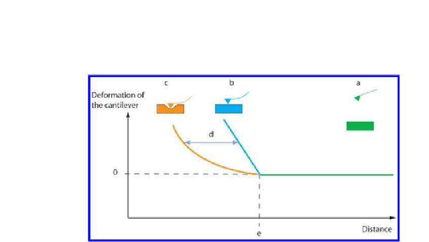
Figure 16.4.
The shapes of two typical indentation curves: one for a hard (b: blue),
and one for a soft (c: orange) sample. The portion of the trace than runs parallel to
the
x
-axis (green) is referred to as the off-contact (a) region, and is common to both
samples. The point of coincidence of the two curves (e) corresponds to the point
of contact between the cantilever tip and the sample. “d” denotes the indentation
distance, which is obtained by subtracting curve c from curve b.
provides information on the stiffness of the sample. Different mathematical
models exist to extract this information from the FD curves. The oldest one,
referred to as the Hertz model, assumes the tip to be spherical, and the sample
to be of ininite dimensions, perfectly lat, isotropic and homogeneous.
This model does not account for the existence of any adhesive, capillary,
electrostatic or magnetic force between the tip and the sample. To obtain
a numerical value of the sample's Young's modulus, the FD curve must be
converted into an indentation curve, which describes the relationship
between the indentation depth of the tip and the cantilever delection. In
other words, the indentation curve describes the force that must be applied
to the tip to push it a given depth into the sample. The indentation curve is
obtained by subtracting the FD curve for a soft sample from the FD curve for
=
3(1 -
ν
2
)
F
____________
4
E
r
1/2
δ
3/2
(16.7)
where
E
is Young's modulus of the sample;
ν
, Poisson's ratio;
F
, Force applied
by the cantilever;
R
, radius of cantilever tip; and
δ
, indentation depth.


Search WWH ::

Custom Search