Geography Reference
In-Depth Information
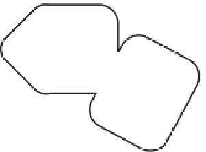
FIGURE 7-5 Polygons to be buffered
FIGURE 7-6 Buffers around polygons
There are many variations on the buffering theme. You can buffer only one side of a line. You can ask
that line buffers have flat ends, in which case areas past the ends of the line are not included in the
buffer. Very importantly, you can buffer features by different thresholds. The thresholds are taken from
information in the attribute table of the feature being buffered. For example, suppose that you wanted to
establish “no smoking” zones around wells. Perhaps your features consist of water wells, oil wells, and
natural-gas wells. You could set things up so that water wells were buffered by 30 meters, oil wells by
100 meters, and gas wells by 400 meters.
Generating Features by Overlaying
Pick any point of Earth's land area. A large number of attributes might describe that point. It may be
within the area owned by a person. The point will be in some country or other. It might be part of a
floodplain. It will have associated with it a certain soil type. The representation of the point in a GIS might
indicate that it is part of a roadway or stream. Or its GIS representation might show it to be an oil well.
In doing GIS analysis, we are frequently interested in combinations of attributes that relate to points,
lines, or areas. For example, we might be interested in those areas that have a certain land use zoning
and that are also for sale. Suppose that we have one GIS layer whose polygons show zoning and another,
different layer that shows properties for sale. By a process called overlaying, we can create a third layer
from which we can identify those properties with the zoning we want that are also for sale.
The term “overlay” comes from the physical process of laying one map of transparent material on top of
another—say, on a light table—and examining the effect of the combination. To continue the preceding
example, suppose that you wanted to buy some property to start a business. The zoning had to be “B1”
and, of course, the property had to be for sale. You might take a clear Mylar map of the area and use a
marker to blacken all of the zones that were not B1. On a second such map, you might blacken all of the
properties that were not for sale. If you then laid both maps on a light table (assuming that they covered
the same area, were at the same scale, were based on the same geographic datum, had the same projection,
and so on—not a trivial assumption as you know by now), light would shine through the areas that might
be suitable for your intended business. With GIS software we can simulate this activity, with much greater
efficiency and garnering much more information in the process. You encountered the essence of overlay,
working the Wildcat Boat problem, when you found combinations of suitable soils and land use.
Let's look first at the idea of overlaying a polygon feature class with another polygon feature class. We
get two types of results: one (geo)graphic and the other tabular.
Figure 7-7 and Table 7-1 depict a feature class named A, consisting of four polygons. In feature class A
there is an attribute named Zone, which has values
p
,
q
,
r
, and
s
, as shown on the diagram and in the table.


Search WWH ::

Custom Search