Geoscience Reference
In-Depth Information
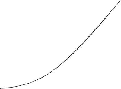
5
Fig. 2.14 Integral form of
the flux-profile
functions for
momentum
Ψ
m
(
ζ
)
and for sensible
heat
Ψ
h
(
ζ
) under
unstable
conditions, as given
by Equations
(2.63) and (2.64).
4
3
Ψ
h
2
Ψ
m
1
0
0.01
0.1
1
10
100
−=− −
0
(
zd L
) /
hypotheses for the entire boundary layer. In this approach, the surface fluxes are commonly
related to “bulk” variables, namely values of the variables at the top and bottom of the ABL,
or their averages over all or part of the ABL. The basic form of the equations is essentially
similar to that of Equations (2.50)-(2.52), or (2.54)-(2.56), but extended for larger heights
aloft above the surface layer. Ideas on the application of similarity to the entire ABL,
including the outer region were put forth early on by Rossby and Montgomery (1935) and
Lettau (1959), and subsequent developments can be traced through the work of Kazanski
and Monin (1961), Clarke and Hess (1974), Zilitinkevich and Deardorff (1974), Yamada
(1976), Garratt
et al.
(1982), Brutsaert (1982), Sugita and Brutsaert (1992), and Jacobs
et al.
(2000), among others. The various versions of this approach can be written in a general
form as follows,
u
k
u
b
=
[ln ((
h
b
−
d
0
)
/
z
0
)
−
B
]
(2.65)
u
k
v
b
=−
A
w
θ
0
ku
∗
θ
s
−
θ
b
=
[ln ((
h
b
−
d
0
)
/
z
0h
)
−
C
]
(2.66)
where
A
B
and
C
are functions of a number of dimensionless variables that affect transport
in the outer region and where the subscript b indicates bulk or characteristic scale variables of
the ABL. Thus
h
b
denotes a characteristic thickness or height scale of the ABL; the variables
u
b
and
v
b
are characteristic horizontal wind velocity components in the
x
- and
y
-directions,
respectively (
x
is the direction of the near-surface wind; because it may involve the Earth's
rotation, usually
y
points to the left of
x
in the Northern Hemisphere, and to the right in the
Southern Hemisphere), such that
u
b
+
v
,
=
V
b
, in which
V
b
is a characteristic wind speed
aloft. These bulk variables have been given different definitions in the past, depending on
the specific implementation of the approach. In the early applications
u
b
,v
b
and
θ
b
were
taken as the values of these variables near the top of the ABL, in general, or just below the
capping inversion, under unstable conditions.
2
b