Geoscience Reference
In-Depth Information
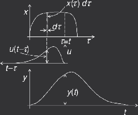
Fig. A5
Illustration of the convolution or
folding operation for a
hereditary or causal system,
with
t
=
0 defined as the start of
the input rate
x
=
x
(
t
). At any
given value of time
t
, the total
output rate
y
is the result (i.e.
integral) of all past inputs from
the start of the input until
t
,
weighted at each instant with the
unit response folded backwards.
In this operation
t
is treated as a
constant and
is the dummy
time variable of the integration.
τ
Equation (A12) describes the output from a system with a memory going back to
.
If the system only has a finite memory
m
, the lower limit of the integral can be changed
to (
t
−∞
−
m
), or
t
y
(
t
)
=
x
(
τ
)
u
(
t
−
τ
)
d
τ
(A13)
t
−
m
Equation (A13) also describes the response of a system, in which the input starts
m
time units prior to
t
. Hence, if the input starts at
t
=
0, the convolution integral
becomes
t
y
(
t
)
=
x
(
τ
)
u
(
t
−
τ
)
d
τ
(A14)
0
In Equations (A12)-(A14),
should be interpreted as the general time variable in the
convolution operation, whereas
t
is the designated time at which the response is to be
determined. The meaning of the name
convolution
or
folding
integral is illustrated for
(A14) in Figure A5.
Because
τ
) in Equations (A11)-(A14), each of these con-
volution integrals can be written in a form which is sometimes more convenient. For
instance, in the case of Equation (A13) this is simply
τ
can be replaced by (
t
−
τ
m
=
u
(
τ
)
x
(
t
−
τ
)
d
τ
(A15)
y
(
t
)
0
and in the case of Equation (A14) it is
t
y
(
t
)
=
u
(
τ
)
x
(
t
−
τ
)
d
τ
(A16)
0