Geoscience Reference
In-Depth Information
10
φ
m
−
1
1
0.1
0.01
0.1
1
10
ζ
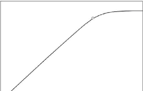
Fig. 2.11 The dependence of (
φ
m
−
1) and (
φ
h
−
1) on
ζ
under stable conditions, as determined in
Cheng and Brutsaert (2005) from experimental wind profile data (circles) and temperature
profile data (triangles) over a flat grassy surface (
z
0
=
110 m) in Kansas in
October, 1999. The solid curve represents Equation (2.60) and the dashed straight line segments
represent Equation (2.57).
0
.
0219 m,
d
0
=
0
.
the basis of the data then available (see Brutsaert, 1982) for stable conditions, the following
was assumed
φ
m
(
ζ
)
=
φ
h
(
ζ
)
=
φ
v
(
ζ
)
=
1
+
5
ζ
for 0
≤
ζ
≤
1
(2.57)
=
6
for
ζ>
1
Equation (2.57) can be integrated with (2.53) to yield the stability correction functions
needed for (2.50)-(2.52). These integral functions are
m
(
ζ
)
=
h
(
ζ
)
=
v
(
ζ
)
=−
5
ζ
for 0
≤
ζ
≤
1
(2.58)
=−
5
−
5ln
ζ
for
ζ>
1
Equations (2.57) and (2.58) can be compared with some more recent experimental data in
Figures 2.11 and 2.12. With these same data a single formulation was proposed by Cheng
and Brutsaert (2005) to cover the entire stable range
ζ
≥
0, namely
m
(
ζ
)
=−
a
ln
ζ
+
(1
+
ζ
b
)
1
/
b
(2.59)
in which
a
and
b
are constants, whose values were found to be
a
=
6
.
1 and
b
=
2
.
5. Equa-
tion (2.59) is also illustrated in Figure 2.12. It can be seen that Equation (2.59) exhibits
nearly the same behavior as the first of Equation (2.58) for small
ζ
, and nearly the same as
the second for large values of
ζ
. The corresponding
φ
-function for the wind profile can be
obtained by differentiation, as indicated by (2.53), to yield
φ
m
(
ζ
)
=
1
+
a
ζ
+
ζ
b
)
−
1
+
1
/
b
ζ
+
(1
+
ζ
b
(1
+
ζ
(2.60)
b
)
1
/
b
As illustrated in Figure 2.11, this equation behaves like (1
+
a
ζ
) for small values of
ζ
and
it approaches a constant (1
+
a
) for large
ζ
, in accordance with (2.57). Figure 2.11 also