Geoscience Reference
In-Depth Information
T
r
1
.0
1
1
.1
1.5
2
3
4
5
10
2
0
50
100
1
4
0
700
5
2
4
3
600
1
9
x
(m
3
s
−
1
)
500
7
400
6
300
4
200
5
100
1
0
−
2
−
1
0
1
2
3
4
5
y
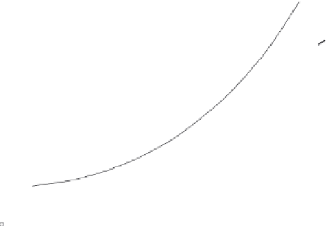
Fig. 13.12 Estimates of the probability distribution of the annual maxima of the rate of flow of the San Pedro
River at Palominas, Arizona, plotted with first asymptotic coordinates. The heavy straight line
(3) represents the first asymptotic distribution for largest values, which was calculated with the first
two sample moments
M
2m
3
s
−
1
; the heavy dashed curve (4)
represents the generalized extreme value distribution calculated with the same moments and with
g
s
=
2m
3
s
−
1
=
180
.
,
and
S
=
115
.
Also shown are the lognormal distribution (thin solid curve 1), the generalized log-gamma
distribution (dashed curve 2), and the power distribution (solid curve 5). Both the
y
1
.
436
.
=
α
n
(
x
−
u
n
)
scale and the
T
r
(
x
) scale (in years) are shown. (See Example 13.8.)
x
=
x
(
T
r
) satisfies
x
(10)
x
(1)
x
(100)
x
(10)
x
(10
n
)
x
(10
n
−
1
)
=
=
= ···=
K
10
(13.82)
where
K
10
is a constant, in which the subscript indicates the ratio of the return periods.
Thus, for the case of, say, a ratio of 2, the magnitude of an event with
T
r
=
2
n
is, by
analogy with (13.82),
K
2
x
(1)
x
(
T
r
)
=
(13.83)
Because
n
=
ln
T
r
/
ln 2, the logarithm of (13.83) can be rewritten as
=
(ln
K
2
/
ln 2) ln
T
r
+
ln
x
(
T
r
)
ln
x
(1)
which immediately results in a power law
aT
r
x
(
T
r
)
=
(13.84)
with the constants
a
ln 2] . Observe that the result obtained in
(13.84) can be derived for any ratio of the return periods. Equation (13.84) with (13.15)
yields the probability distribution function
=
x
(1) and
b
=
[ln
K
2
/
a
)
−
1
/
b
F
(
x
)
=
1
−
(
x
/
(13.85)