Geoscience Reference
In-Depth Information
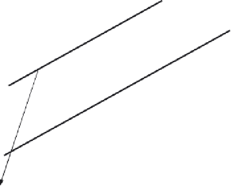
Fig. 10.13 Sketch illustrating the
application of Equation
(10.16) to calculate the
rate of drawdown of the
water table (WT), when
treated as a free
surface. The
equipotentials are lines
of constant hydraulic
head
h
. (After Kirkham
and Gaskell, 1951.)
B
water table
A
equipotential
θ
B
'
C
streamline
β
D
A
'
equipotential
Example 10.1. Displacement of a free surface
The physical significance and the application of Equation (10.16) can be illustrated for the
situation shown in Figure 10.13. An infinitesimally small portion of the water table AB
moves along the streamlines AA
and BB
to a new position A
B
during a short increment
of time
the angle between the streamlines and
the vertical, then it can be seen that the vertical component of the distance of the water table
fall AD is given by
δ
t
.If
β
is the slope of the water table and
θ
AC
=
AA
(cos
θ
−
sin
θ
tan
β
)
(10.19)
According to Darcy's law the total distance traveled by the point A during
δ
t
is
n
e
∂
h
k
0
AA
=−
∂
s
δ
t
(10.20)
where
∂
h
/∂
s
is the hydraulic gradient along AA
. Substitution of Equation (10.20) into
(10.19) with the observation that
∂
h
∂
s
∂
h
∂
z
∂
h
∂
s
∂
h
∂
x
cos
θ
=
and
sin
θ
=
(10.21)
results in
∂
h
∂
x
k
0
n
e
tan
β
−
∂
h
∂
z
AC
=
δ
t
(10.22)
This result, which was first derived by Kirkham and Gaskell (1951), is essentially a finite
difference form of Equation (10.16).
10.2.2 Some features of free surface flow solutions
Probably the earliest solution of this type of problem was presented by Kirkham and Gaskell
(1951) for the very similar flow situation of a falling water table during tile and ditch