Geoscience Reference
In-Depth Information
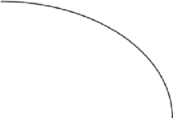
Fig. 9.4
Sketch illustrating the
calculation of the
infiltrated volume
F
as
the area under the
θ
=
θ
(
z
) curve, that is
the water content
profile in the soil at a
given instant in time
t
.
This can be done by
integrating either the
elemental area (
zd
θ
)or
the elemental area
(
θδ
z
θ
0
z
δθ
δθ
dz
). The coordinate
z
points down into the
soil;
z
θ
θ
i
0 is where the
water infiltrates, and
z
=
z
f
is the position of
the wetting front.
=
z=0
δ
z
z=z
f
in which
x
is used instead of
z
to indicate the absence of gravity in the present case. With
the solution in terms of the Boltzmann variable (9.11), this assumes the form
θ
0
t
1
/
2
F
=
φ
d
θ
(9.16)
θ
i
The integral in this equation has constant limits and is therefore also a constant. Thus, for
conciseness of notation it is often convenient to express horizontal infiltration in terms
of the sorptivity, defined by Philip (1957a) as
θ
0
A
0
=
φ
θ
d
(9.17)
θ
i
The cumulative infiltration (9.16) can now be written as
A
0
t
1
/
2
=
F
(9.18)
=
/
and the rate of infiltration
f
dF
dt
1
2
A
0
t
−
1
/
2
f
=
(9.19)
The point here is that both equations indicate unequivocally how horizontal infiltration
capacity proceeds in time, even though the solution is left unspecified so far.
Note that, because that solution can also be written as
θ
=
θ
(
φ
), the rate of infiltration
t
−
1
/
2
,
can be expressed alternatively as a Darcy flux, or because
∂φ/∂
x
=
x
=
0
=−
φ
=
0
D
w
∂θ
∂
D
w
d
θ
t
−
1
/
2
f
=−
(9.20)
x
d
φ