Geoscience Reference
In-Depth Information
( b )
( a )
0 . 3
0 . 3
θ
θ
0 . 2
0 . 2
0 . 1
0 . 1
0
0
−
1 0 0
−
8 0
−
6 0
−
4 0
−
2 0
0
−
1 0 0
−
8 0
−
6 0
−
4 0
−
2 0
0
ψ
w
=
p
w
/
γ
w
( c m )
ψ
w
=
p
w
/
γ
w
( c m )
( d )
( c )
0 . 3
0 . 3
0 . 2 5
0 . 2 5
θ
θ
0 . 2
0 . 2
0 . 1 5
0 . 1 5
0 . 1
0 . 1
0 . 0 5
0 . 0 5
−
3 0
−
2 0
ψ
w
=
p
w
/
−
1 0
0
−
3 0
−
2 0
ψ
w
=
p
w
/
−
1 0
0
γ
w
( c m )
γ
w
( c m )
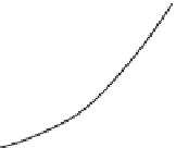
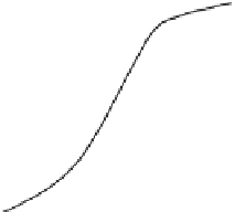
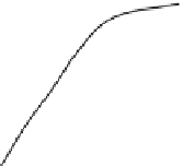
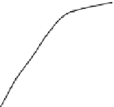
Fig. 8.14 Soil water characteristic relationship showing hysteresis with boundary and primary scanning curves
for (a) Adelaide dune sand, draining; (b) Adelaide dune sand, wetting; (c) Molonglo sand, draining;
and (d) Molonglo sand, wetting. The lines are best-fit through the data;
ψ
w
denotes pressure expressed
as equivalent water column. (After Talsma, 1970.)
presented of hysteresis for different sandy soils. The bounding curves of the hysteresis
regions shown in these figures are called
wetting and drying boundary curves
; any point
inside the hysteresis region can be reached by scanning curves; the scanning curves
starting from the drying and wetting boundary curves can be called
primary wetting and
drying scanning curves
, respectively. It is obvious by now that there is an infinity of
possible scanning curves in the hysteresis region. To describe these quantitatively, some
type of interpolation scheme must be devised.