Geoscience Reference
In-Depth Information
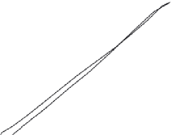
Fig. 7.9
Storage in the channel reach
S
(m
3
hs
−
1
), as a function of
the weighted flow rate
XQ
i
+
(1
−
X
)
Q
e
(m
3
s
−
1
)for
values of
X
=
0.1 (triangles),
0.3 (circles), and 0.5
(squares) with the values of
the flow rates of Example
7.2, listed in Table 7.2.
4 0 0 0
S
3 0 0 0
2 0 0 0
1 0 0 0
0
0
1 0 0 0
2 0 0 0
XQ
i
+ ( 1
-
X) Q
e
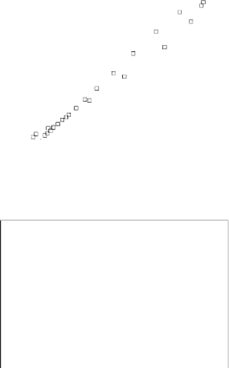
Fig. 7.10 Observed
hydrographs at the
inflow end
Q
i
and at
the outflow end
Q
e
(in m
3
s
−
1
) listed
in Table 7.2, and
used in Example 7.2
(heavy solid lines).
The calculated
outflow hydrograph,
shown as a dashed
line, is obtained
with the
Muskingum method
with
X
=
0.3
and
K
=
1.99 h.
2000
Q
i
Q
e
Rate
of
flow
1000
0
0
5
10
15
20
25
30
Time (h)
=
X
0.3 appeared to yield the best single valued relationship, required by (7.15). This is
illustrated in Figure 7.9; also shown are the curves for the extreme values
X
0.1 and
0.5 to illustrate the evolution of the relationship as a function of
X
. The regression line
in the form of (7.15) for the value of
X
=
489. (This
suggests that initially the storage in the reach could have been assumed to be
S
=
0.3 is
S
=
1.99 (0.3
Q
i
+
0.7
Q
e
)
−
=
489
m
3
hs
−
1
, instead of the value
S
0 adopted in Table 7.2, in order to force the regression
in Figure 7.9 through the origin in accordance with Equation (7.15)). The time of travel
through the reach is
K
=
=
1.99 h. With these values of
X
and
K
, Equation (7.37) can be
written as
Q
e2
=−
0.472
Q
e1
; the calculated outflow hydrograph
can be compared in Figure 7.10 with the original data of
Q
e
(i.e. the values listed in Table
7.2) used in the calibration.
0.051
Q
i2
+
0.579
Q
i1
+