Geoscience Reference
In-Depth Information
1
0.8
q
L
+
0.6
0.4
0.2
0
0
0.2
0.4
0.6
0.8
1
1.2
1.4
t
+
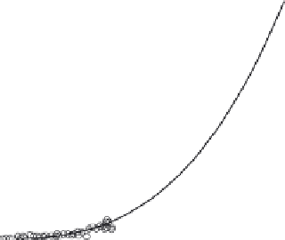
Fig. 6.7
Comparison between scaled rising hydrograph obtained with the kinematic wave approach (for
laminar flow with
a
=
2) and scaled experimental data obtained by Izzard (1944) on a plane covered
with asphalt. The solid line represents
q
L
+
=
t
3
+
. The data points come from several different
experimental combinations, namely rainfall intensities
P
=
i
=
91.4 and 45.7 mm h
−
1
, slopes
S
0
=
0.001, 0.005, 0.01 and 0.02, and plane lengths
L
=
22, 15, 7.3 and 3.7 m. (After Morgali, 1970.)
B
1
1
t
+
=
0
B
2
h/h
sL
0.2
B
3
0.5
0.5
t =1
B
4
+
A
1
A
2
A
3
A
4
t
+
=5
B
5
C
0
0
0.2
0.4
0.6
0.8
1
x/L
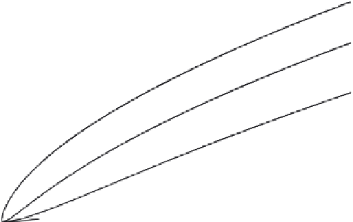
Fig. 6.8 Water depth profiles 0A
1
B
1
C, 0A
2
B
2
C, etc., during the decay phase, obtained with the kinematic
wave approach (with
a
3) ; the profiles are shown as functions of downstream distance at
different times after the cessation of the lateral inflow
i
. The water depth is normalized with the
equilibrium depth at
x
=
L
, which is given by Equation (6.19) or
h
s
L
=
(
iL
/
K
r
)
1
/
(
a
+
1)
. The initial
profile is the equilibrium, i.e. steady state, profile shown in Figure 6.4. The characteristic starting at A
1
successively passes A
2
,A
3
, etc., and maintains a constant
h
, until it is swept off the plane at
x
=
L
.
=
2
/