Geoscience Reference
In-Depth Information
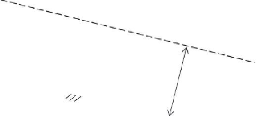
Fig. 5.6 Sketch of the
decomposition of
the water depth
variable as
h
=
h
0
+
h
p
, for the
purpose of
linearization;
h
0
is a
steady uniform flow,
and
h
p
=
h
p
(
x
,
t
)is
a small disturbance.
h
p
h
h
0
Solutions of the dynamic part
If the departures
V
p
and
h
p
are assumed to be small, one can, as a further approximation,
neglect the effect of the additional turbulence resulting from the perturbation, and put
S
f
=
S
0
. This leaves then only the purely dynamic part of the momentum equation, i.e. the
first three terms of the second of Equations (5.44). Differentiating the second of (5.44) with
respect to
x
, and eliminating (
∂
V
p
/∂
x
) by means of the first, one can combine these two
equations into one, or in the absence of lateral inflow,
2
h
p
∂
2
h
p
t
+
V
0
−
gh
0
∂
2
h
p
∂
∂
+
2
V
0
∂
=
0
(5.45)
t
2
∂
x
∂
x
2
Because the undisturbed flow is uniform and steady, it is convenient to describe the motion of
the small disturbance relative to a reference moving with the velocity
V
0
of this undisturbed
flow. This can be done by substituting
x
m
=
t
, where the subscript m
refers to the moving reference; thus the partial derivatives are
∂/∂
x
=
∂/∂
x
m
and (
∂/∂
t
)
=
(
∂/∂
t
m
)
−
V
0
(
∂/∂
x
m
), and Equation (5.45) becomes
(
x
−
V
0
t
) and
t
m
=
∂
∂
t
m
−
gh
0
∂
2
h
p
2
h
p
∂
x
m
=
0
(5.46)
Similarly, by differentiating the first of (5.44) with respect to
x
, substituting (
∂
h
p
/∂
x
) from
the second of (5.44) and by using the same coordinate transformation, one obtains
∂
∂
t
m
−
gh
0
∂
2
V
p
2
V
p
∂
x
m
=
0
(5.47)
The same type of equation can also be derived for the rate of flow
q
=
Vh
. Putting
q
=
q
0
+
q
p
, one has
q
0
=
V
0
h
0
and
q
p
=
V
0
h
p
+
V
p
h
0
, because
V
p
h
p
is negligible. Thus one obtains,
by adding Equations (5.46) and (5.47), after multiplying each by
V
0
and
h
0
, respectively,
2
q
p
∂
2
q
p
∂
∂
t
m
−
gh
0
∂
x
m
=
0
(5.48)
Equations (5.46), (5.47) and (5.48) are in the form of the classical linear wave equation
2
y
2
y
∂
x
m
=
0
∂
∂
t
m
−
c
0
∂
(5.49)