Performance-Based Seismic Design - Structural Seismic Design Optimization and Earthquake Engineering - page 44

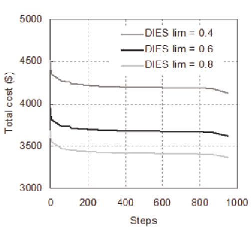
Figure 9. Influence of the cost-damage relationship used

characteristics. This model is commonly known
as BWBN (Bouc, 1967; Baber et al., 1981, 1985).
The objective in this second application is a
comparison of the influence that the two differ-
ent hysteretic modeling techniques have in either
reliability assessment or structural optimization.
The pile has a diameter D = 0.356 m , with
wall thickness t = 0.10 m , and a length L = 30 m .
Yield strength and elastic modulus of the steel
were assumed deterministic and to have nominal
values (respectively, 250 Mpa and 200000 Mpa ).
Twenty earthquake records were simulated as sta-
tionary processes using a spectral representation
based on the Clough-Penzien power spectrum
density function (Clough and Penzien, 1975), an
envelope modulation function (Amin and Ang,
1968), and twenty different sequences of random
phase angles.
For different combinations of the intervening
variables, databases were constructed for the
mean response Δ and its standard deviation over
the twenty records. These databases were then
used to train corresponding neural networks, as

previously discussed. Finally, the response Δ in
Eq.(49) was represented by using the lognormal
format and the error representation as shown in
Eqs.(44) and (34).
The pile was subjected to the displacement
history Δ( t ) in Figure 11. The finite element ap-
proach was used to calculate the hysteresis loop in
Figure 12. This response was used to calibrate the
parameters of a BWBN model, with the resulting
loop shown in Figure 13.
Dynamic analyses for the different earthquake
records were carried out with either the BWBN
representation of the hysteretic restoring force or,
alternatively, calculating each time the hysteresis
via the finite-element model. In both cases, the
neural network methodology previously described
was applied.
Table 10 shows the statistical data assumed
for the intervening variables, and Table 11 the
reliability results obtained for different values of
the capacity factor λ.
The parameters ω S and T define, respectively,
the Clough-Penzien power spectrum density func-