Life Cycle Cost Considerations in Seismic Design Optimization of Structures - Structural Seismic Design Optimization and Earthquake Engineering - page 17

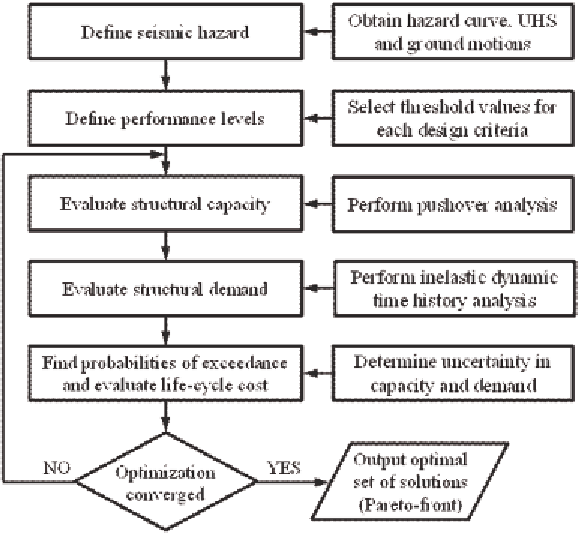
Figure 9. Steps for performing LCC oriented seismic design optimization

ground motion is selected for each return period
(see the section “The LCC Model” for more in-
formation) and spectrum matching (Abrahamson,
1993) is used to achieve direct correspondence
between the records and the hazard levels. The
acceleration response spectra of the records after
spectrum matching are shown in Figure 11(b).
The life-time of the structure, t , is considered
as 50 years. The cost of repair for the IO, LS, and
CP limit states, C i , are taken as 30, 70 and 100
percent of the initial cost of the structure based
on the correspondence of the limit states defined
previously and the information provided by Fra-
giadakis et al. (2006b). The hazard curve as a
function of PGA is shown in Figure 11(a). The
functional form in Eqn. (8) is fitted to the hazard
curve to allow for the numerical integration of
Eqn. (3). The demand side of fragility relationship
given in Eqn. (4), i.e. the first term, as a function
of PGA, is obtained by finding the maximum
interstory drift under the three hazard levels
through inelastic dynamic analysis and it is rep-

resented analytically by curve fitting to mathe-
matical form in Eqn. (6). The dispersion in
earthquake demand, β D , is quantified as 0.25, 0.35
and 0.45 for the three hazard levels with 75, 475
and 2475 years return period, respectively, by
running additional analysis. The details of this
derivation are omitted here for the sake of brev-
ity. As mentioned earlier, the structural limit states
are also established by carefully investigating
different design alternatives in the search space
by conducting pushover analysis and considering
local response measures, i.e. strains in the longi-
tudinal reinforcement and concrete core. The
structural capacity is evaluated for a range of
design variables and the mean values for the three
limit states IO, LS and CP are obtained as 0.4%,
2% and 3.5% interstory drift. The uncertainty in
capacity is assumed to be equal to 0.35 taking
previous research as a reference (Wen, et al.,
2004). First the conditional probability (fragility)
in Eqn. (4), then the total probability in Eqn. (3)
is calculated. The damage state probabilities are