Life Cycle Cost Considerations in Seismic Design Optimization of Structures - Structural Seismic Design Optimization and Earthquake Engineering - page 14

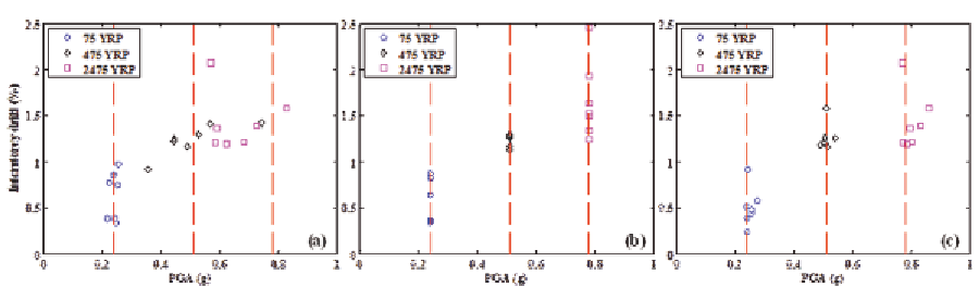
Figure 7. Dispersion in earthquake demand for different representations of the earthquake hazard using:
(a) natural, (b) scaled, and (c) spectrum compatible records

The Optimization Algorithm respectively, of earthquake demand evaluated

using inelastic dynamic analysis. The mean and
standard deviation are the parameters of the cor-
responding normal distribution that describes
the earthquake demand. The curve fitting to the
earthquake demand obtained from the spectrum
compatible records that are mentioned above for
the mean and standard deviation using the first
option in Eqn. (6) and Eqn. (7), respectively, is
shown in Figure 8.
The hazard curve can also be described in
mathematical form

A brief review of most commonly used optimiza-
tion algorithms is provided above. The objectives
of the optimization problem considered here are
highly nonlinear (due to the inelastic dynamic
analysis that is used to predict earthquake de-
mand) and the derivatives with respect to the
design variables are discontinuous. Furthermore,
the design variables (i.e. section sizes and rein-
forcement ratios) are discrete. Therefore, the use
of gradient-based optimization algorithms is not
well suited. The evolutionary algorithms have
shown to be very efficient in solving combinatorial
optimization problems as reviewed above. Here,
the taboo search (TS) algorithm is selected and
discussed in more detail. The same algorithm is
also used to obtain the optimal solutions for the
example application provided in the next section.
TS algorithm, first developed by Glover (1989,
1990), then it is adapted to multi-objective opti-
mization problems by Baykasoglu et al. (1999a,
1999b). An advantage of TS algorithm is that a set
of optimal solutions (Pareto-front or Pareto-set)
could be obtained rather than a single optimal
point in the objective function space. The meth-
odology presented in Baykasoglu et al. (1999a,
1999b) is used here with further modifications as
described below.

( ) = ⋅

c IM ⋅ c ⋅ IM

v IM c e + ⋅ c e (8)

8 10

7 9

where c 7 through c 10 are constant to be determined
from curve fitting to the hazard curve.
With the above described formulation each
term in Eqn. (3) is represented as an analytical
function of the ground motion intensity, IM . Thus,
using numerical integration the desired probabili-
ties of Eqn. (2) can easily be calculated. The cost
of repair for the IO, LS, and CP limit states, C i ,
are usually taken as a fraction of the initial cost
of the structure. Finally, the LCC is evaluated
through Eqn. (1).