Overall Conceptual Seismic Design and Local Seismic Capacity Design for Components of Bridges - Structural Seismic Design Optimization and Earthquake Engineering - page 288

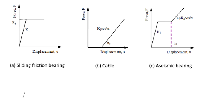
Figure 15. Stiffness models

The axial stiffness of a cable member is defined
as K

cables, u 0 denotes the design free displacement
when the bearing is in normal service load and
α is the angle between the longitudinal direction
of the cable when engages at a lateral displace-
ment of u 0 and the direction of the horizontal
relative displacement of the friction bearing. So
combined with the characteristics of the fric-
tional bearing and the cables, the integral stiffness
model of the cable sliding friction aseismic bear-
ing can be shown in Figure 15c, where n is the
number of cables and ϕ is a coefficient that
represents the equivalent linearization of cable
stiffness under severe earthquakes.
Depending on pseudo-static cyclic loading
experiments and finite element analyses for a
prototype cable sliding friction aseismic bearing
(Figure 16) where the maximum vertical load is
5000 kN, the actual values of the bearing's char-
acteristics, such as the static and dynamic friction
coefficients of the bearing's sliding surface, the
cable stiffness, the experimental hysteretic curves
of the bearing and the corresponding skeleton
curves, can be obtained (Cao, 2009; Yuan, Cao,
Cheung, Wang & Rong, 2010). The experimental
results show that the static and dynamic friction
coefficients decrease as the vertical load increas-
es. Through the experiments and calculations, the
coefficient ϕ is suggested to be 0.373 for its ap-
plication in theoretical analysis models of the new

2 1 = , where E is the elastic modulus of
the cables, A 1 is the cable section area and L is
the cable length.

EA L

2. Shear strength of the bolt

Considering the requirements under service
loads, the horizontal shear resisting capacity of
the fixed-type pot bearing should not be less than
10% of the vertical load bearing capacity (Cao,
2009). Depending on the performance objects,
the shear bolt should be out of service during
severe earthquakes. So it is suggested that the
shear strength of the bolt be within 10% to 15%
of its vertical load capacity.

3. Integral stiffness of the bearing

The lateral stiffness of a frictional bearing can
be simplified as an ideal bilinear model as shown
in Figure 15a, where K 1 denotes the elastic stiff-
ness of the bearing and F s denotes the critical
friction force which is calculated as F

s = µ where
µ is the friction coefficient and N is the vertical
force on the bearing. The cables can be regarded
as completely elastic material since they should
not yield, whose load-displacement curve is shown
in Figure 15b, where K 2 is the stiffness of the

N