Life Cycle Cost Considerations in Seismic Design Optimization of Structures - Structural Seismic Design Optimization and Earthquake Engineering - page 13

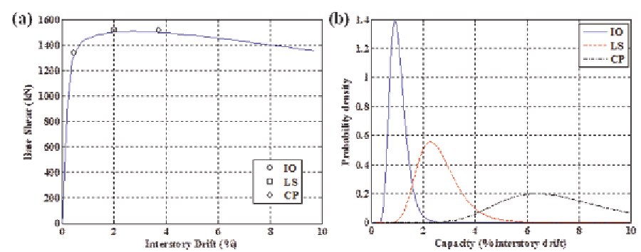
Figure 6. (a) A typical pushover curve and the limit state points that delineate the performance levels,
(b) illustration of lognormal probability distributions for the three structural limit states (IO: immediate
occupancy, LS: life safety, CP: collapse prevention)

most studies they are taken as constants due to
lack of information.
The dispersion in earthquake demand (here
represented with β D ) due to variability in ground
motions is established here using a simple struc-
tural system (2-story 1-bay RC frame) and three
sets of earthquake ground motions each represent-
ing a different hazard level at return periods of
75, 475 and 2475 years. Each set includes seven
ground motions which are selected from the PEER
database (PEER, 2005) to represent the hazard at
a selected site in San Francisco, CA (more details
are given in the example application below). The
correspondence between the hazard levels and the
ground motions is achieved using three different
methods. In the first method, the natural records
are used without any modification. In the second
method, the records are scaled based on PGA to
match the PGA of the respective hazard level (in
this case 75, 475 and 2475 years return period
earthquakes are represented with a PGA of 0.24 g,
0.51 g and 0.78 g, respectively). And in the third
method, spectrum matching is used to make the
acceleration response spectrum of each record
compatible with the UHS corresponding to each
return period shown in Figure 3(b). The results

are shown in Figure 7. It is seen that although the
mean of demand from three different methods
are similar, a higher dispersion is obtained when
natural and scaled ground motions are used.
The dispersion also increases with increasing
ground motion intensity (i.e. earthquake return
period). The focus of this chapter is optimal
seismic design of structures considering the LCC
(not assessment); therefore, the use of spectrum
compatible records is suggested. For assessment
purposes, the use of unmodified (natural) records
is recommended.
The mean, µ D , and standard deviation, σ D , of
earthquake demand, as continuous functions of
the ground motion intensity could be described
using (Aslani & Miranda, 2005)

( ) = ⋅

c c

µ D IM c IM or c c

IM

⋅ IM (6)

2 3

1 1 2

( ) = + ⋅

2

σ D IM c c IM c + ⋅ IM (7)

4 5 6

where the constants c 1 through c 3 and c 4 through
c 6 are determined by curve fitting to the data
points that match the PGA of the ground motions
records with the mean and standard deviation,