Applications of Topology Optimization Techniques in Seismic Design of Structure - Structural Seismic Design Optimization and Earthquake Engineering - page 247

subsequently ∆ x from Equation (1.53). Like the
single modal case, to find the value of the Lagrange
multiplier Γ an inner bisection loop can be used.
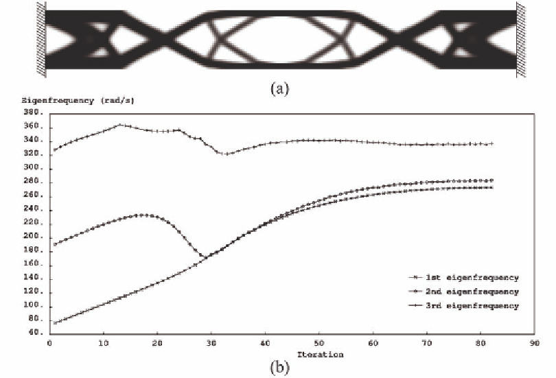
Figure 7 shows the final solution and the evolu-
tion history of the first three eigenfrequencies of the
problem of example 2 using the above approach.
It can be seen that the multiple eigenvalues evolve
smoothly and a better solution is achieved.
Table 1 compares the final value of the first
three eigenfrequencies of example 2 obtained
using the three approaches considered here. As
expected, using the multiple eigenvalue sensi-
tivities yields the best result.

than increasing them. For an objective function
defined as a combination of natural frequencies,
the optimization problem can usually be addressed
by minimal modification of the eigenfrequency
maximization problem. Typically one just needs
to update the sensitivities. One example of such
objective functions was defined in Equation (1.33)
and dealt with in the preceding section. Other
examples include maximizing the gap between
two natural frequencies (see e.g. Du and Olhoff
2007 and Zhao et al. 1997) or designing structures
with a specified set of frequencies or eigenmode
shapes (see e.g. Xie and Steven 1996, Yang et al.
1999b, Maeda et al. 2006) among others.
A common practical case is where the excitation
frequency is known and it is desired to move the
natural frequencies as far away as possible from
the excitation frequency. A suitable objective
function can be defined as

6. CONTROLLING THE NATURAL
FREQUENCIES

In dynamic design of structures one usually re-
quires to control the natural frequencies rather

Figure 7. Solving example 2, using multiple eigenvalue sensitivities: final solution (a) and evolution of
the first three eigenfrequencies (b)