Graphics Reference
In-Depth Information
v
i
c
c
v
i
-1
v
i
-1
H
i
H
i
(a)
(b)
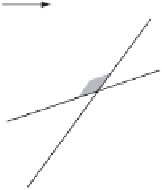
Figure 9.8
(a)
v
i
−1
is contained in
H
i
, and thus
v
i
=
v
i
−1
. (b)
v
i
−1
violates
H
i
, and thus
v
i
must lie somewhere on the bounding hyperplane of
H
i
, specifically as indicated.
be some other feasible point on the segment between
v
i
and
v
i
−
1
more extreme in
direction
c
than
v
i
, leading to a contradiction).
v
i
therefore can be found by reducing
the current LP problem to
d
1 dimensions as follows. Let
c
be the projection of
c
−
into
π
. Let
G
i
be the intersection of
H
j
,1
≤
j
<
i
, with
π
. Then,
v
i
is the solution to
−
the
d
1-dimensional LP problem specified by the
G
i
constraints and the objective
vector
c
. Thus,
v
i
can be solved for recursively, with the recursion bottoming out
when
d
1. In the 1D case,
v
i
is trivially found as the largest or smallest value
(depending on the direction of
c
) satisfying all constraints. At this point, infeasibility
of the LP problem is also trivially detected as a contradiction in the constraints.
To start the algorithm, an initial value for
v
0
is required. Its value is obtained by
means of introducing a bounding box
P
0
large enough to encapsulate the intersection
volume
P
. Because an optimum vertex for
P
remains an optimum vertex for
P
0
∩
=
P
, the
problem can be restated as computing, at each iteration, the optimum vertex
v
i
for
the polyhedron
P
i
=
H
i
(from
v
i
−
1
of
P
i
−
1
of the previous iteration).
The initial value of
v
0
now simply corresponds to the vertex of
P
0
most extreme in
direction
c
(trivially assigned based on the signs of the coordinate components of
c
).
It is shown in [Seidel90] that the expected running time of this algorithm is
O
(
d
P
0
∩
H
1
∩
H
2
∩···∩
m
).
Seidel's algorithm is a
randomized algorithm
[Mulmuley94], here meaning that the
underlying analysis behind the given time complexity relies on the halfspaces initially
being put in
random
order. This randomization is also important for the practical
performance of the algorithm.
Figure 9.9 graphically illustrates Seidel's algorithm applied to the triangles from
Figure 9.7. The top left-hand illustration shows the six original halfspaces. The next
seven illustrations show (in order, one illustration each)
P
0
through
H
6
being pro-
cessed. At each step, the processed halfspace
H
i
is drawn in thick black, along with the
v
i
for that iteration. With the given (random) ordering of the halfspaces, three recur-
sive 1D calls are made: for halfspaces
H
2
,
H
5
, and
H
6
. For these, the 1D constraints
in their respective bounding hyperplane are shown as arrows.
!