Graphics Reference
In-Depth Information
C
K
BL
J
D
G
D,E,F,G,H,I
A
FH
A,B,C,J,K,L
E
I
D,E F
G,H,I
A,B,C
J,K,L
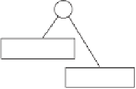
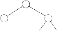
Figure 8.4
First steps of the construction of a leaf-storing BSP tree, using the same geometry
as before.
These two halves are then divided again, at which point the construction is stopped,
in that a reasonable partitioning has been obtained. Leaf-storing BSP trees (along
with
k
-d trees, quadtrees, and octrees) are common collision geometry data structures,
in particular when the collision geometry is given as a polygon soup.
8.2.3
Solid-leaf BSP Trees
Unlike the previous two BSP tree types, solid-leaf BSP trees are built to represent the
solid volume occupied by the input geometry. That is, dividing planes are ultimately
selected to separate the solid volume from the exterior of the object. A 2D example
is shown in Figure 8.5, in which a solid-leaf BSP tree is constructed to represent the
interior of a concave (dart-shaped) polygon.
Note that the supporting plane of every polygon in the input geometry must be
selected as a dividing plane or the object's volume will not be correctly represented.
Specifically, the dividing plane immediately before a leaf node always corresponds
to a supporting plane. However, other internal tree nodes can use arbitrary dividing
planes, allowing for a better balancing of the tree. In fact, for the object in Figure 8.5
a better BSP tree could be constructed by starting with a dividing plane through the
concave vertex and its opposing vertex.
Note also that no geometry is stored in the tree. The leaf nodes only indicate
whether the remaining area in front and behind of the dividing plane is empty or solid.
In other words, a solid-leaf BSP tree can be seen as partitioning the input volume
into a collection of convex polyhedra, which are then represented as the intersection
volume of a number of halfspaces. The dividing planes of the BSP tree correspond to