Biomedical Engineering Reference
In-Depth Information
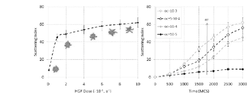
FIGURE 2.12: Left panel: scattering index of 16 MLP-29 cell clusters after
3000 MCS ( 24 h) as a function of the HGF secretion rate . Insets are
representative configurations after 3000 MCS. Right panel: comparison of time
evolution of S
I
for
c
= 10
5
s
1
,
c
= 10
4
s
1
, 510
4
s
1
, and 10
3
s
1
.
All standard deviations are evaluated over over 10 simulations.
a quasi-Gaussian profile, as it levels off toward the clusters boundary, while
its inection point is at the cell{cluster boundary.
The analysis of the dynamics of single individuals permits one to charac-
terize in greater detail the differentiation of cells in the aggregate: those in the
sprouts, after the polarization, have a persistence motion in the direction of
the branch they belong to, whereas the others (in the valley or in the center)
keep a round shape and have a more isotropic dynamic, as shown in Figure
2.11. In particular, it is useful to emphasize that the anisotropic migration re-
quires no extra assumptions in the CPM and produces long persistence time
in the presence of HGF cues, because, as seen, cells change direction slowly.
The long persistence time introduces two time scales into the branching mor-
phogenesis: the faster time scale along the longer axes produces the growth
of the spikes, and the slower time scale, radially directed, coarsens the main
corpus of the island.
To have a deeper idea of the quantity of HGF needed for sprouting and
to test whether its dose affects the results, the simulation model is run with
increasing values of
c
(i.e., = "
c
), while the other parameters are unchanged.
The initial island does not sprout for
c
< 10
4
s
1
, requiring a minimal level
of HGF to start the process, while above this value a sort of phase transition
is observed (see Figure 2.12), and the branching process regularly develops.
The tendency of cells to polarize, elongate, and have a persistent dynamics
affects the geometry of the branches. This is studied running a set of simula-
tions keeping the same initial configuration as that in Figure 2.9 and gradually
increasing
per
C
(the other parameters are unchanged, with
c
= "
c
= 510
4
s
1
). For 1 <
per
C
< 45 the sprouts become longer and thinner with an al-
most linear trend respect to the
pers
C
increments. In fact, for very low values


Search WWH ::

Custom Search