Characterizing Aquifers - Hydrogeology: Objectives, Methods, Applications - page 136

They are done with a constant discharge over a period of 1 to 3 days,
possibly more for long-term testing, and require the creation of a peripheral
piezometer network. Monitored parameters include the pumped discharge
and the level of the water table in the pumping well and in the piezometers.
One can also observe the rise of the water table in the pumping well and in
the piezometers as soon as pumping is stopped (Figure 73).
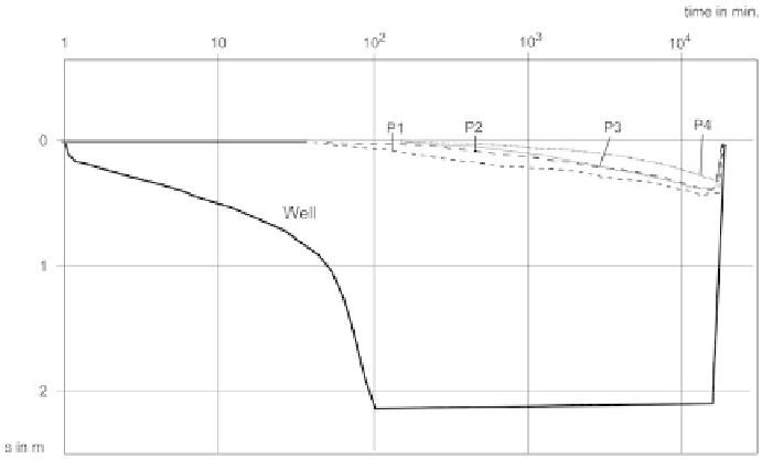
Figure 73 Example of a pumping test. Alluvial aquifer of the Loup River (Alpes-Maritimes).
The pumping data are graphed, with time, t, in logarithmic abcissa
(in hours, minutes, or seconds), and the drawdown, s, or the residual
drawdown, sr (for the rise), on a linear scale (in meters or centimeters).
The data points create a representative curve for the test, the fi rst part
of which shows the well's capacity, and whose alignment along a straight
line would represent a test in an unlimited aquifer.
The transmissivity, T, can be calculated with Jacob's logarithmic
approximation method:
T = 0.183 ⋅ Q/c,
where Q is the pumping discharge (in m 3 ·h -1 ) and c is the slope of the
line.
The storativity, S, determined from piezometric curves, is given by the
following equation:
S = (2.25 ⋅ T⋅ t 0 )/x 2 ,
where T is transmissivity (in m 2 ·s -1 ), t 0 is the time of intersection between
the drawdown (or recharge) curve and the initial piezometric level (in s),