Geography Reference
In-Depth Information
Distances from objects: buffers
4.5
In applications where selection of objects within a set distance of other objects is the
concern, generation of a buf er polygon is a likely step. Buf ers are widely used in site-
selection projects and in many other contexts where straight line (Euclidean) distances
are meaningful. Cases where distance is more logically measured along networks (as
would be the case when the distance between places by road is measured), rather than
as a straight line between start and end points, are dealt with in Chapter 6.
4.5.1
Vector buffers
A buf er polygon represents the area within a specii ed distance of an object—that is,
if the buf er is computed for a distance of 5 km, the buf er polygon represents a dis-
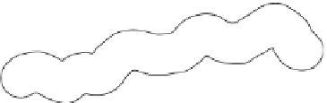
tance of 5 km from the object of interest. Figure 4.2 gives an example of a buf er poly-
gon around a linear feature. h e object could also be a point (in which case, the buf er
is a circle) or a polygon. Overlay operators, which could be used to identify areas or
objects falling within buf er polygons, are discussed in Chapter 5.
One method for generating buf ers entails moving a circle with the required radius
along the feature to be buf ered. h e internal boundaries of the overlapping circles can
then be dissolved (see Section 4.10 for a discussion about dissolving internal boundar-
ies). Ot en, buf ers are computed for several distance bands and items that fall within
each band can be identii ed using an overlay operator, as detailed in the following
chapter. Such an operation is routine in most GIS sot ware. It is also possible to vary
the width of the buf er to take into account specii c local characteristics. For example,
buf ers may be wider in areas with steep slopes or in areas that are environmentally
sensitive.
4.5.2
Raster proximity
Buf ers can also be represented as raster grids. For an input of cells that are coded as
locations of interest, a buf er grid can be generated. In such an output, cells within the
specii ed distance of the objects will be given one value (e.g. 1) while cells outside
of that area will be given another value (e.g. 0). With the raster model, proximity is
ot en measured directly and each cell in the output records the distance from the cell
or cells of interest in the input grid. Figure 4.3A shows such a grid with cell values
representing the distance of cells from a linear feature running from the top let to
the bottom right of the grid—the feature corresponds to the cells with zero distance
Figure 4.2
Buffer (polygon with light line) around a linear feature (heavy line).


Search WWH ::

Custom Search