Spatial interpolation - Spatial Data Analysis: An Introduction for GIS Users - page 153

(see Section 9.7.2 for a discussion about this). h e use of a i tted model for interpola-
tion is detailed in the next subsection. In this case, the geostatistical sot ware Gstat
(Pebesma and Wesseling, 1998; Pebesma, 2004) was used for the analysis; ArcGIS™
Geostatistical Analyst could also be used (although the variogram will appear slightly
dif erent given the way the semivariances are computed in that package).

9.10.2 Interpolation

Precipitation amounts were predicted on a regular grid using the IDW, TPS, and OK
functions of ArcGIS™ Geostatistical Analyst. For OK, the variogram was estimated
using a lag size of 5000 and 20 lags, with the model (nugget ef ect = 403.9, spherical com-
ponent (partial sill) = 14689, and range = 90653.3 m) i tted using Geostatistical Analyst.
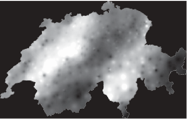
Figure 9.16 shows a grid generated using the 16 nearest neighbours with IDW.
Cross-validation was used to compare the three methods using 16 nearest neigh-
bours. When using cross-validation to compare prediction approaches, it is usual to
use summaries of the errors such as the mean error or the RMSE. As its name suggests,
the RMSE is the root of the mean squared errors (i.e. take each error, square it, take the
average of these squared errors, and then take the square root of this average); this is a
widely used summary measure and is interpreted below. h e mean error indicates bias:
if it is negative then the procedure tends to under-predict values and when it is positive

Precip itation (1/10 mm)
High : 582.097

Low : 0.029

0 50 100 km

Figure 9.16 Precipitation on 8 May 1986: IDW prediction using 16 nearest neighbours.