Spatial interpolation - Spatial Data Analysis: An Introduction for GIS Users - page 144

compared irrespective of the direction in which they are aligned—that is, whether
they are aligned (approximately or absolutely) on a line north-south or east-west, etc.
of one another is irrelevant. A variogram computed from data in all directions is
termed 'omnidirectional.
In Figure 9.10, the semivariance values tend to be smaller for small lags and they
generally increase with an increase in lag size until perhaps 25,000 m, where the values
tend to level out (this is demonstrated below). h is indicates that values are positively
spatially autocorrelated up to approximately this distance. At distances larger than
this, there is no spatial structure. h e variogram provides a useful means of summariz-
ing how values change with separation distance. Using topography as an example, data
representing a 'smooth' surface like a l ood plain will have a very dif erent variogram
to data representing a 'rough' surface like a mountain range.
A mathematical model may be i tted to the experimental variogram and the coef-
i cients of this model can be used for spatial prediction using kriging or for condi-
tional simulation (dei ned below). A model can be i tted 'by eye' or by using some
i tting procedure such as ordinary least squares (see Sections 3.3 and 8.5, and Appendix
E) or weighted least squares. A model is usually selected from one of a set of 'autho-
rized' models. Webster and Oliver (2007) provide a review of some of the most widely
used authorized models.
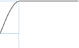
h ere are two principal classes of variogram model. Transitive (bounded) models
have a sill (i nite variance)—that is, the variogram levels out as it reaches a particular
lag. Unbounded models do not reach an upper bound. Figure 9.11 shows the compo-
nents of a bounded variogram model. h ese will be dei ned and then practical exam-
ples given. h e nugget ef ect, c 0 , represents unresolved variation (a mixture of spatial
variation at a i ner scale than the sample spacing and measurement error). h e struc-
tured component, c , represents the spatially correlated variation. h e sill (or sill vari-
ance), c 0 + c , is the a priori variance. h e range, a , represents the scale (or frequency) of
spatial variation. For example, if a region is mountainous and elevation varies mark-
edly over quite small distances, then the elevation can be said to have a high frequency
of spatial variation (a short range), while if the elevation is quite similar over much of
the area (e.g. it is a river l ood plain) and varies markedly only at the extremes of the

Range ( a )

Total sill ( c 0 + c )

γ( h ) Sill ( c )

Nugget ( c 0 )

Lag (h)

Figure 9.11 Bounded variogram model.