Geography Reference
In-Depth Information
Legend
Observations
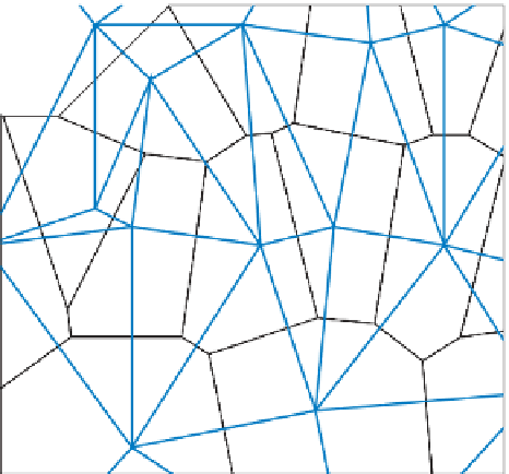
TIN
Thiessen polygons
Figure 9.3
TIN subset with Thiessen polygons superimposed.
h e illustrations here are based on the
V
variable derived from elevation data and
described by Isaaks and Srivastava (1989). For the purposes of their example, Isaaks
and Srivastava refer to the variable
V
as concentrations of some material in parts per
million (ppm), here the variable is expressed in the same way, although the data are
treated as elevation values for illustrative purposes. h e data are used as they are pref-
erentially sampled and allow the illustration of the TIN and some of its potential
benei ts in terms of smaller data storage requirements relative to an altitude matrix.
Figure 9.4 shows the point data, a raster grid generated with IDW (with an expo-
nent of 2 and using eight nearest neighbours), and the edges of triangular facets derived
using Delaunay triangulation. h e TIN was generated using ArcGIS™ 3D Analyst.
Figure 9.5 shows a '2.5D' visualization of the TIN. In this case the 'elevations' are
multiplied by 0.04 with respect to the
x
and
y
coordinate values, which has the ef ect
of compressing the 'elevation' values. h e ridge of large values running along the west
of the region from north to south is apparent in Figure 9.5.
Regression for prediction
9.4
Regression (whether a global or local variant, like geographically weighted regression)
can be used for spatial interpolation if values of the independent variable are available
at all locations where predictions are required. In the previously outlined case of eleva-
tion and precipitation amount, if we have a DEM with elevation values at all locations
in the study area then we can use the regression equation (either globally or locally) to
predict precipitation amounts for all grid cell locations in the DEM (see, for example,
Lloyd, 2005).


Search WWH ::

Custom Search