Graphics Reference
In-Depth Information
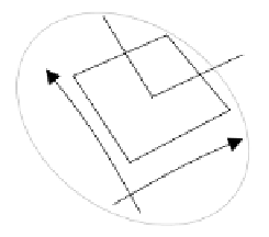
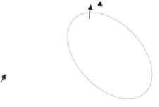
∂
P
∂v
N
∂
P
∂u
v
P
u
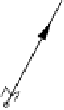
Figure 10.6.
The next step is to effectively displace the surface along
N
by a value stored in a bivariate
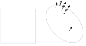
scalar function (bump map) F uv. Figure 10.7(a) shows such a map indexed by u and v.
Figure 10.7(b) shows a surface defined by a bivariate vector function
P
uv with some of its
normal vectors. Figure 10.7(c) shows the perturbed surface
P
uv after its normal vectors
have been disturbed by F uv.
F
(u,v)
v
u
P
(u,v)
P
′
(u,v)
(a)
(b)
(c)
Figure 10.7.
Before the displacement is performed,
N
is normalized to keep the process consistent:
N
N
Thus, the displaced point
P
is defined as
N
P
=
P
+
F
N
These new points form the secondary perturbed surface that is rendered. But the renderer
requires access to the surface normals associated with
P
, which is defined using
P
u
×
P
v
N
=
(10.7)
The partial derivatives in Eq. (10.7) are expanded using the chain rule:
F
N
N
P
u
=
P
u
+
F
u
N
+
N
u