Graphics Reference
In-Depth Information
and the transform becomes
⎡
⎣
⎤
⎦
=
⎡
⎣
⎤
⎦
·
⎡
⎣
⎤
⎦
x
p
y
p
z
p
a
2
K
+
−
+
x
p
y
p
z
p
cos
abK
c sin acK
b sin
abK
+
c sin
2
K
+
cos
bcK
−
a sin
acK
−
b sin bcK
+
a sin
2
K
+
cos
where K
cos .
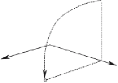
To test this transform, let's perform a simple rotation such as rotating the point P 110 90
about the x-axis
=
1
−
n
ˆ
=
i
. With reference to Fig. 7.2, it is obvious that the answer is P
101.
Y
P
(1,1,0)
Z
X
P
′(1,0,1)
Figure 7.2.
If
=
90
, then K
=
1
−
cos 90
=
1. Also, if the axis of rotation is
n
ˆ
=
i
, then a
=
1b
=
0, and
c
=
0. Therefore, the transform becomes
⎡
⎤
⎡
⎤
⎡
⎤
1
0
1
100
000
010
1
1
0
⎣
⎦
=
⎣
⎦
·
⎣
⎦
which is correct.
7.3 Complex numbers
Complex numbers were discovered in the 16th century but were not fully embraced by mathe-
maticians, who tended to endorse their “imaginary” associations. Eventually, in the early 19th
century, Carl Friedrich Gauss [1777-1855] showed that complex numbers had a geometric
interpretation, and the mathematical landscape was prepared for a fertile period of discovery.
Prior to the discovery of complex numbers, it was difficult to manipulate the square
roo
t of
a negative number. However, with the invention of
i
, which could stand in place of
√
−
1, the
imaginary world of complex numbers came into being.
By definition, a complex number z has the form
z
=
a
+
i
b or z
=
a
+
b
i
where a and b are real quantities and
i
2
=−
1. The position of
i
is not important, and in this
text it is placed after the scalar. An example is 2
+
3
i
, where the real part is 2 and the imaginary