Evolving Neural and Fuzzy Systems - Computational Intelligence in Time Series Forecasting - page 302

For evolving the network architecture, there are also two alternative approaches
available:

x evolving the pure network architecture , without interconnecting weights,
which presumes that weight values are to be determined through network
training
x simultaneous evolution of both architecture and weights.

8.1.1.3 Evolving the Pure Network Architecture
Evolving a genuine network architecture requires a decision about the degree to
what extent the genotypes ( i.e. the chromosomes) should bear the detailed
information related to the targeted network architecture. This depends on the
representation scheme to be used. Should it be a direct representation that includes
all the details of every node, or should it be an indirect representation in which
only some dominant nodes are represented by some details like the number of
hidden layers and the number of neurons in the layers?

6

000110
000100
000010
000001
000001
000000

4 5

1

2 3

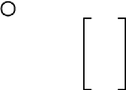
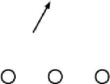
Figure 8.2. Example of low level encoding

If the genotypes should not contain any statements about the connecting
weights, then a random set of initial weight values can be taken. In this case the
risk exists that the weight values finally determined could be noise spoiled. This is
because the fitness values of genotypes will be represented by fitness values of
phenotypes, which could be due to the randomization of initial values of training
runs (Angeline et al. , 1994). To reduce this noise the use of one-to-one mapping
between the genotypes and phenotypes is recommended ( McDonnel et al ., 1994).
Otherwise, when using the direct encoding scheme in evolving the pure
network architecture, each network connection is represented by a binary string of
a specified length. Once accepted for representation, the strings should be
concatenated to build corresponding chromosomes . The set of chromosomes
belonging to the same network can then form the connectivity matrix that itself
depicts the network architecture in terms of network interconnection pattern. This
is shown in Figure 8.2. The matrix, again, could also be interpreted in the inverse