Memory - Computational Explorations in Cognitive Neuroscience - page 274

and 1 otherwise (think of it as a binary distance or error
measure computed on the names).
The sum of the closest event distances over the epoch
of training is plotted in yellow in the graph log. As
the network starts producing outputs that exactly match
valid outputs in the environment (though not necessarily
the appropriate outputs for the given input pattern), this
should approach zero. Instead of plotting the sm_nm
statistic, the graph log shows both_err , plotted in
blue. Like sm_nm , this compares the closest event
name with the actual input name, but this one looks only
at the part of the event name that identifies the input pat-
tern (i.e., the portion of the name before the _ charac-
ter). Thus, it gives a 1 if the output is wrong for both
possible outputs. This, too, should approach zero as the
network trains.
As something of an aside, it should be noted that
the ability to learn this one-to-many mapping task de-
pends critically on the presence of the kWTA inhibition
in the network — standard backpropagation networks
will learn to produce a blend of both output patterns
instead of learning to produce one output or the other
(cf. Movellan & McClelland, 1993). Inhibition helps by
forcing the network to choose one output or the other,
because both cannot be active at the same time under the
inhibitory constraints. We have also facilitated this one-
to-many mapping by adding in a small amount of noise
to the membrane potentials of the units during process-
ing, which provides some randomness in the selection
of which output to produce. Finally, Hebbian learning
also appears to be important here, because the network
learns the task better with Hebbian learning than in a
purely error driven manner. Hebbian learning can help
to produce more distinctive representations of the two
output cases by virtue of different correlations that exist
in these two cases. O'Reilly and Hoeffner (in prepara-
tion) provides a more systematic exploration of the con-
tributions of these different mechanisms in this priming
task.
Having trained the network with the appropriate “se-
mantic” background knowledge, we are now ready to
assess its performance on the priming task.

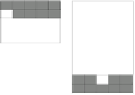
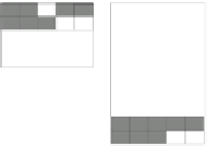
Output

Input

0_b 1_b 2_b

Output

Input

0_a 1_a 2_a

Figure 9.2: Six sample input (bottom) - output (top) patterns
for training. Events 0 a and 0 b have the same input pattern,
but map to two different output patterns, producing a one-to-
many (two) mapping.

First, do View , TRAIN_LOG to get a graph log of
training progress. Do Train in the control panel to start
training — you can see the network being trained on
the patterns. Then, turn off the Display in the network
speed the process.
The graph log shows two statistics of training. As
with the Reber grammar network from chapter 6 (which
also had two possible outputs per input), we cannot
use the standard sum_se error measure (which target
would you use when the network can validly produce
either one?). Instead, we use a closest event statistic to
find which event among those in the training environ-
ment has the closest (most similar) target output pat-
tern to the output pattern the network actually produced
(i.e., in the minus phase). This statistic gives us three re-
sults, only one of which is useful for this training phase,
but the others will be useful for testing so we describe
them all here: (a) the distance dist from the closest
event (thresholded by the usual .5), which will be 0 if
the output exactly matches one of the events in the en-
vironment; (b) the name of the closest event ev_nm ,
that does not appear in the graph log because it is not
a numerical value, but it will appear on our testing log
used later; (c) sm_nm that is 0 if this closest event has
the same name as that of the event currently being pre-
sented to the network (i.e., it is the “correct” output),

Iconify the training graph log. Press View on the
wt_prime_ctrl control panel and select TEST_LOGS .