Perception and Attention - Computational Explorations in Cognitive Neuroscience - page 243

activity correlates with LGN patterns of activity. If the
V2 unit reliably responds to only one input pattern, the
resulting activation based receptive field will just be that
input pattern. If the V2 unit responds equally to a set of
ten input patterns, the result will be the average of these
ten patterns. The corresponding mathematical expres-
sion for a given receptive field element r i (correspond-
ing to an LGN unit i , in the example above) is:

(8.1)

( t ) x ( t )

( t )

where yj ( t ) is the activation of the unit whose recep-
tive field we are computing (the V2 unit in the example
above), xi ( t ) is the activation of the unit in the layer on
which we are computing the receptive field (LGN in the
example above), and t is an index over input patterns, as
usual. Note that this is very similar to what the CPCA
Hebbian learning rule computes, as we saw in the pre-
vious simulation. However, as in the V2-LGN example
above, we can use the activation based receptive field
procedure to compute “weights” (receptive field values)
for layers that a given unit is not directly connected to.
For example, it can also be useful to look at a unit's
activation based receptive field by averaging over the
output images, to see what object the unit participates
in representing.
Now, let's take a look at the activation based receptive
fields for the different layers of the network.

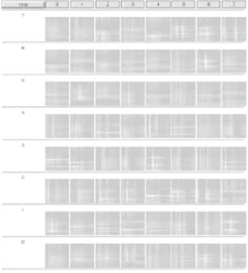
Figure 8.13: V2 activation-based receptive fields from on-
center LGN inputs. The large-scale 8 x 8 grid represents one
hypercolumn's worth of units, with each large grid containing
a grid representing the on-center LGN input. The colors repre-
sent the values of the activation-weighted averages over input
patterns. The neurons appear to represent low-order conjunc-
tions of features over a (small) range of locations.

Press View on the overall control panel, and se-
lect ACT_RF .Press Open in the file selection window to
pull up the input receptive field for the V2 units from the
on-center LGN layer (figure 8.13). Another file selection
window will also appear; you can move that aside while
you examine the current display.
Because we are doing weight sharing, we need only
look at one hypercolumn's worth of V2 units, which are
displayed in the large-scale 8 x 8 grid in this window.
Within each of these grid elements is another grid rep-
resenting the activation-weighted average over the input
patterns, which is the activation based receptive field for
this unit. Note that these units are in the first (lower
left hand) hypercolumn of the V2 layer, so they receive
from the corresponding lower left hand region of the
input, which is why the receptive fields emphasize this
region.

, !

Notice that some units have brighter looking (more
toward the yellow end of the scale) receptive fields and
appear to represent only a few positions/orientations,
while others are more broadly tuned and have dimmer
(more toward the dark red end of the scale) receptive
fields. The brightness level of the receptive field is di-
rectly related to how selective the unit is for particu-
lar input patterns. In the most selective extreme where
the unit was activated by a single input pattern, the re-
ceptive field would have just maximum bright ri = 1
values for that single pattern. As the unit becomes
less selective, the averaging procedure dilutes the re-
ceptive field values across all the patterns that the unit
represents, resulting in dimmer values. We can use