Combined Model and Task Learning, and Other Mechanisms - Computational Explorations in Cognitive Neuroscience - page 193

the (often delayed) effects of these actions. The goal
of the organism is naturally to produce actions that re-
sult in the maximum total amount of reward. Because
the organism cares less about rewards that come a long
way off in the future, we are typically interested in dis-
counted future rewards. This can be expressed mathe-
matically in terms of the following value function :

(6.3)

where V (t) expresses the value of the current state or
situation at a given point in time. ￿ (between 0 and 1)
is the discount factor that determines how much we ig-
nore future rewards, r(t) is the reward obtained at time

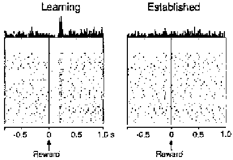
Figure 6.18: Changes in VTA firing with learning (display as
in previous figure). During learning, firing occurs only during
the delivery of the reward. After acquisition of the task has
been established, firing does not occur when the reward is ac-
tually delivered, and instead occurs after the instruction stim-
ulus as shown in the previous figure.

(where time is typically considered relative to some
defining event like the beginning of a training trial), and
the h:::i brackets denote the expectation over repeated
trials. Because ￿ is raised to the power of the future
time increments, it gets exponentially smaller for times
further in the future (unless ￿ =1 ).
Equation 6.3 plays a role in TD much like that of
the sum-squared error (SSE) or the cross-entropy error
(CE) in error-driven learning algorithms — it specifies
the objective of learning (and is thus called the objec-
tive function for TD learning). Whereas in error driven
learning the goal was to minimize the objective func-
tion, the goal here is to maximize it. However, it should
become rapidly apparent that maximizing this function
is going to be rather difficult because its value at any
given point in time depends on what happens in the fu-
ture . This is just the same issue of temporally delayed
outcomes that we have discussed all along, but now we
can see it showing up in our objective function.
The approach taken in the TD algorithm to this prob-
lem is to divide and conquer. Specifically, TD divides
the problem into two basic components, where one
component (the adaptive critic, AC ) learns how to es-
timate the value of equation 6.3 for the current point in
time (based on currently available information), while
the other component (the actor ) decides which actions
to take. These two components map nicely onto the two
components of the basal ganglia shown in figure 6.16a,
where the striosomes play the role of the adaptive critic
and the matrisomes correspond to the actor. Similarly,
the ventromedial frontal cortex might be the adaptive
critic and the dorsal frontal cortex the actor.

Schultz et al. (1993).

delivered, but after acquisition of the task has been es-
tablished, firing occurs for the predictive stimulus, and
not to the actual reward.
Thus, VTA neurons seem to fire whenever reward can
be reliably anticipated, which early in learning is just
when the reward is actually presented, but after learn-
ing is when the instruction stimulus comes on (and not
to the actual reward itself). This pattern of firing mir-
rors the essential computation performed by the TD al-
gorithm, as we will see. Note that this anticipatory fir-
ing can be continued by performing second order con-
ditioning , where another tone predicts the onset of the
original tone, which then predicts reward. VTA neurons
learn to fire at the onset of this new tone, and not to the
subsequent tone or the actual reward.

6.7.1 The Temporal Differences Algorithm

Now, we will see that the properties of the temporal
differences algorithm (TD) (Sutton, 1988) provide a
strong fit to the biological properties discussed earlier.
The basic framework for this algorithm (as for most re-
inforcement learning algorithms) is that an organism
can produce actions in an environment , and this en-
vironment produces rewards that are contingent upon