Error-Driven Task Learning - Computational Explorations in Cognitive Neuroscience - page 147

this time, the output units are not clamped, but are in-
stead updated according to their weights from the input
units (which are clamped as before). Thus, the testing
phase records the actual performance of the network on
this task, when it is not being “coached” (that is why it's
atest).
The results of testing are displayed in the test grid log
that was just opened. Each row represents one of the 4
events, with the input pattern and the actual output ac-
tivations shown on the right. The sum_se column re-
ports the summed squared error (SSE), which is sim-
ply the summed difference between the actual output
activation during testing ( o k )andthe target value ( t k )
that was clamped during training:

Event_2 Event_3

Event_0 Event_1

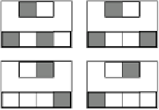
Figure 5.3: The hard pattern associator task mapping, where
there is overlap among the patterns that activate the different
output units.

Let's see what the network has learned.

Turn the network Display back on, and press the
TestStep button 4 times.
This will step through each of the training patterns
and update the test grid log. You should see that the
network has learned this easy task, turning on the left
output for the first two patterns, and the right one for
the next two. Now, let's take a look at the weights for
the output unit to see exactly how this happened.

, !

(5.1)

where the sum is over the 2 output units. We are ac-
tually computing the thresholded SSE, where absolute
differences of less than .5 are treated as zero, so the unit
just has to get the activation on the correct side of .5 to
get zero error. We thus treat the units as representing un-
derlying binary quantities (i.e., whether the pattern that
the unit detects is present or not), with the graded acti-
vation value expressing something like the likelihood of
the underlying binary hypothesis being true. All of our
tasks specify binary input/output patterns.
With only a single training epoch, the output unit is
likely making some errors.

Click on r.wt in the network window, and then on
the left output unit.
You should see that, as expected, the weights from
the left 2 units are strong (near 1), and those from the
right 2 units are weak (near 0). The complementary
pattern should hold for the right output unit.

, !

Question 5.1 Explain why this pattern of strong and
weak weights resulted from the CPCA Hebbian learn-
ing algorithm.

Now, turn off the Display button in the up-
per left hand side of the network window, then open
a graph log of the error over epochs using View ,
TRAIN_GRAPH_LOG . Then press the Run button.
You will see the grid log update after each epoch,
showing the pattern of outputs and the individual SSE
( sum_se ) errors. Also, the train graph log provides a
summary plot across epochs of the sum of the thresh-
olded SSE measure across all the events in the epoch.
This shows what is often referred to as the learning
curve for the network, and it should have rapidly gone
to zero, indicating that the network has learned the task.
Training will stop automatically after the network has
exhibited 5 correct epochs in a row (just to make sure
it has really learned the problem), or it stops after 30
epochs if it fails to learn.

, !

Now, let's try a more difficult task.

Set env_type on the pat_assoc_ctrl control
panel to HARD , and Apply . Then, do View , EVENTS .
In this harder environment (figure 5.3), there is over-
lap among the input patterns for cases where the left
output should be on, and where it should be off (and the
right output on). This overlap makes the task hard be-
cause the unit has to somehow figure out what the most
distinguishing or task relevant input units are, and set
its weights accordingly.
This task reveals a problem with Hebbian learning.
It is only concerned with the correlation (conditional
probability) between the output and input units, so it

, !