Geology Reference
In-Depth Information
thickness and with apparent sand thickness (defined
as the trough-to-peak time separation). It is evident
that the character of the tuning curve is related to the
shape of the wavelet (
Fig. 3.16b
), with the actual
thickness vs amplitude relationship having a shape
similar to a wavelet half cycle. The amplitude tuning
curve is a maximum at the sand thickness below
which the peak and trough separation remains con-
stant. This is commonly referred to as the tuning
thickness. Below the tuning thickness, the amplitude
decreases in response to the thinning sand.
A comparison of
Figs. 3.16b
,
c
indicates that, for a
limited range of thicknesses above tuning thickness,
estimating sand thickness using trough-to-peak sep-
aration would result in a slight underestimate. Note
that although tuning imposes limits on the interpret-
ation of thicknesses the changes in seismic amplitude
and apparent thickness can be used in net pay inter-
pretation (
Chapter 10
).
Interference related to two reflections of the same
polarity is shown in
Figs. 3.16e
,
f
. In this model the
two reflections converge to a single loop at the tuning
thickness. The tuning thickness is characterised by
maximum destructive interference (i.e. low ampli-
tude) and as the wedge thins below this point there
is an increase in amplitude. This type of interference
pattern might
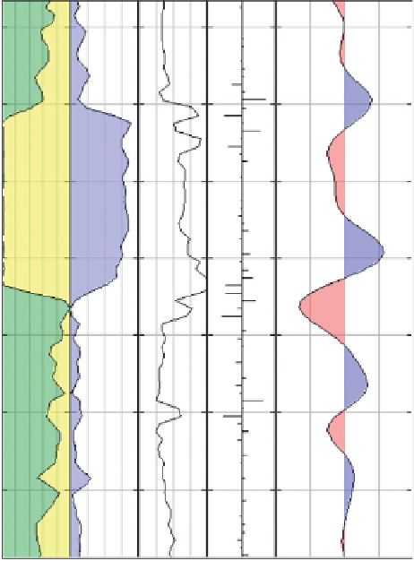
V
sh
Phi
AI
Rc
Synthetic
0
1 0
0.4
4
8
-0.2
0.2 0.25
0.25
be
characteristic
of
angular
unconformities.
Figure 3.15
Synthetic seismogram illustrating how geology relates
to seismic.
3.7.3 Estimating vertical resolution
from seismic
For practical purposes the tuning thickness can be
considered as an indication of the vertical
resolution. Fundamentally, the tuning thickness is
determined by the compressional velocity of the unit
and the wavelength of the seismic pulse (
shale) such that the reflection coefficients at top and
base of the wedge are equal but of opposite polarity.
It is particularly applicable for example to isolated
gas sands in unconsolidated basin fill sections.
Figure 3.16
(upper part) shows an example of this
type of model constructed using a positive standard
polarity zero phase wavelet. The figure shows the
modelled seismic response together with crossplots
of thickness and amplitude, and illustrates the key
problem for vertical resolution (in the sense of
uniquely identifying the top and base of the wedge).
Owing to the finite seismic bandwidth there is a
thickness below which the seismic loops effectively
have a constant separation. Thus, when the sand is
very thin, estimating its thickness from the separation
of trough and peak seismic loops will result in a
significant overestimate (
Fig 3.16c
).
The tuning curves in
Figs. 3.16b
,
c
show how the
trough amplitude changes with both actual sand
). A first
order approximation for making quick calculations:
λ
tuning thickness
¼ λ=
4
ð
Widess, 1973
Þ
ð
3
:
3
Þ
λ ¼
V
p
ð
m
=
s
Þ=
F
d
ð
Hz
Þ
ð
3
:
4
Þ
F
d
¼
1
=
T,
ð
3
:
5
Þ
where
λ ¼
wavelength (m), F
d
¼
dominant frequency
and T
(measured in seconds from trough
to trough or peak to peak) on a seismic section
(e.g.
Fig. 3.17
).
¼ '
period
'
33
A worked example based on
Fig. 3.17
: