Geology Reference
In-Depth Information
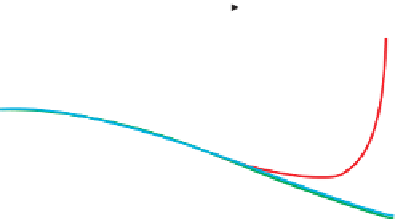
Usual range of seismic acquisition angles
Figure 2.19
Comparison of Aki-
Richards two-term and three-term
equations and Hilterman equation for an
example interface of a shale overlying a
gas sand.
0.2
Aki-R 2 term
Aki-R 3 term
Hilt. approx
0.1
0
-0.1
-0.2
-0.3
-0.4
-0.5
-0.6
0
10
20
30
40
50
60
70
Incidence angle
V
p
V
s
AI
PR
ρ
Shale
Gas sand
2438
1006
2.25
5486
0.397
2600
1700
1.85
4810
0.127
highlight the fact that reflectivity is fundamentally
related to two rock properties, the acoustic impedance
contrast and the Poisson
is less helpful if there is complicated layering or grad-
ational change in properties across a boundary.
s ratio contrast (see
Chapter
5
for rock property controls on acoustic impedance
and Poisson
'
2.3.4.2 Wedge model
The wedge model (
Fig. 2.20b
) is a tool to describe
the interaction of reflections from two converging
interfaces, and is therefore an important way to under-
stand interference effects. In particular the wedge
model is useful for determining vertical resolution
(
Chapter 3
) and can also be used in simple approaches
to net pay estimation (
Chapter 10
). However, like the
single interface model the wedge model can be too
simplistic for practical purposes, particularly in areas
where there are rapid vertical variations in lithology.
'
s ratio).
2.3.4 Types of seismic models
There are a number of different types of models that
can be generated to aid amplitude interpretation (
Fig.
2.20
). For most applications these utilise relatively
simple primaries-only reflectivity. However, there
may be occasions when more sophisticated modelling
is required. The key problem is that as the complexity
or sophistication increases, the time and effort also
increases, often without any guarantees that it will be
worth the effort. The user needs to select the right
degree of complexity for the problem at hand.
2.3.4.3 1D synthetics based on log data
The synthetic seismogram uses wireline log data and a
wavelet to calculate either a single normal incidence
trace or a range of traces at different angles, simulat-
ing the angle variation in a seismic gather. This type
of model is important when tying wells to seismic
(
Chapter 4
) and when generating multi-layered
models with different fluid fill. One-dimensional
(1D) synthetic models are useful in understanding
how the seismic response depends on the frequency
content of the data (
Chapter 3
). Following the
response of a layer of interest from the fully resolved
case with a (perhaps unrealistic) high-bandwidth
wavelet through the increasingly complex interference
patterns that may arise as the bandwidth decreases is
2.3.4.1 Single interface model
The simplest model (and sometimes the most import-
ant aid to understanding) is the single interface
model, where V
p
, V
s
and
for the upper and lower
layers are input into an algorithm based on Zoeppritz
or its approximations to produce the AVO plot,a
graph of reflection coefficient versus incidence angle
(
Fig. 2.20a
). This is often the best place to start. If the
target comprises thick layers with significant contrasts
at top and base, this simple model will give a good
idea of what to expect in real seismic data. However, it
ρ
17