Geology Reference
In-Depth Information
a)
b)
c)
%
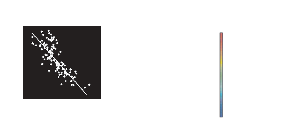
Cross correlation = -0.79
AI
40
36
10000
30
30
24
20
8000
18
10
5000
12
7000 9000 11000
Average AI (m/sec.g/cc)
6000
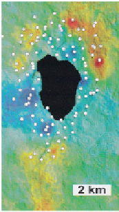
Figure 10.11
.,
1996
; copyright 1996, SPE. Reproduced with permission of SPE. Further
reproduction prohibited without permission). (a) Crossplot of average porosity from wells vs average seismic impedance for the upper part
of the Tor chalk formation, (b) average seismic impedance map, (c) porosity map generated from collocated cokriging. Note that the centre of
the map is data-free owing to the presence of a gas cloud (colour illustrations from Dubrule,
2003
).
Ekofisk Field porosity mapping (after Doyen
et al
with fine sampling over a large lateral extent. Alter-
natively, information derived from seismic attributes
can be used to define the lateral variability. Tech-
niques such as collocated cokriging and kriging with
external drift are examples of kriging that combine
seismic attribute data with well data and provide
a single deterministic solution that fits the wells.
Kriging with external drift is usually applied in depth
conversion as there is an implicit assumption that the
secondary variable (e.g. stacking velocities) provides
low frequency information on the primary variable
(e.g. average velocity). Collocated cokriging effectively
provides a weighted average of the kriged estimate (in
which a spatial co-variance or variogram model is
specified) and the estimate derived from the linear
regression of the rock property and seismic attribute.
The weighting factor is related to the correlation
coefficient between the seismic attribute and the res-
ervoir property (Doyen et al.,
1996
;
Fig. 10.11
).
estimating hydrocarbon in place. For example, one
approach might be to use data from a deterministic
inversion, with hydrocarbon sand thickness esti-
mated from a relationship between impedance and
hydrocarbon pay. As described in
Chapter 9
,this
approach requires a large number of wells to under-
stand the various effects of smoothing and residual
tuning effects that may bias the estimation. Stochas-
tic inversion techniques may address these pitfalls
but these also require good well control and may not
be practical in exploration scenarios. Fortunately,
there are relatively simple approaches that may be
applicable, dependent on the geology, for inferring
hydrocarbon pay sand thickness from seismic and
these can be utilised readily with commonly available
software.
10.3.4.1 Amplitude scaling techniques
Simple techniques for hydrocarbon pay estimation
can be applied in situations where the reservoir is an
isolated low impedance unit of limited thickness
(generally less than about 60 ms; Brown et al.,
1984
,
1986
; Connolly,
2007
). These techniques effectively
assume a bi-polar arrangement of sand and shales,
each with a single value of impedance, with net sand
being predicted from mapped seismic amplitude by
using the following assumptions:
(1) there is a first order linear relationship between
N:G and amplitude for a given apparent thickness
(
Chapter 5
);
10.3.4 Net pay estimation from seismic
The interpreter has a number of choices when decid-
ing on a technique for interpreting hydrocarbon in
place. Traditional approaches are based on gross
rock volume calculations from depth structure maps.
Stock Tank Oil Initially In Place (STOIIP) or Gas
Initially In Place (GIIP) can then be calculated by
making assumptions about porosity, thickness, net
to gross ratio (N:G), and formation volume factor.
It is possible, however, to use seismic directly for
230